PDF

Secondary Flow in a Semicircular Duct
Introduction
In this example, the Single-Phase Flow, SSG-LRR interface is used to compute fully developed turbulent flow in a semicircular duct. The characteristics of the resulting secondary flow are analyzed and visualized in detail.
Model Definition
The properties of turbulent flows cannot be fully described by eddy-viscosity models. For more exact and complete predictions, differential Reynolds stress models are needed, since they self-consistently account for the turbulence anisotropy, system rotation, and flow curvature. A convenient practical example is given by duct flows with noncircular cross section. In such ducts, turbulence Reynolds stresses lead to secondary circulation in the cross-stream plane with typical velocities of approximately 1%–2% of the bulk streamwise velocity. More convex walls (and sharper corners) attract the secondary flow streamlines, while more concave walls (and blunter corners) repel them.
Here, the semicircular duct from Ref. 1 is investigated. Its height and width are H = 33 mm and W = 94 mm, respectively. The Reynolds number,
is Re = 80,000. Here, Ub is the streamwise bulk velocity and Dh is the hydraulic diameter of the duct.
Computing a fully developed solution (including accurately resolved secondary flow) from an isotropic turbulence state would require the streamwise length to be at least L = 100 Dh. In this study, only a stationary solution is of interest, so it is sufficient to use a Periodic Flow Condition with a very short streamwise geometry dimension.
Figure 1: The computational domain of the semicircular duct, which is at least 700 times shorter than would be needed to achieve a fully developed state from the inlet with isotropic turbulence. Positive z-axis points in the streamwise direction.
Implementation in COMSOL Multiphysics
Figure 1 shows the geometry with the streamwise length l, which is 700 times shorter than L defined above, as well as the boundary conditions. For a duct, the number of numerical iterations needed to propagate high turbulent viscosity from the duct walls to the duct center is approximately independent of the mesh (coarse or fine). Thus, the solution is obtained subsequently on Mesh 1, Mesh 2, and Mesh 3 shown in Figure 2 (continuing from the previously converged solution). Notice that skipping Mesh 1 or Mesh 2 or both increases the overall solution time.
Figure 2: Mesh 1 (coarse), Mesh 2 (normal), and Mesh 3 (fine) used in the model (only two cells in the streamwise direction).
The details of the implementation of the Single-Phase Flow, SSG-LRR interface can be found in the CFD Module User’s Guide; see the section “Theory for the Turbulent Flow Interfaces”.
Results and Discussion
Figure 3: Secondary flow pattern in the cross-stream plane. Streamlines (top) and arrow surface (bottom).
All the results shown below are those obtained on Mesh 3. Mesh dependence can be analyzed using the model file.
Figure 3 illustrates the cross-stream streamlines in the model. Four vortices are formed with those near the flat wall being stronger. The streamlines are attracted by the corners and repelled by the bottom and top walls. The maximum magnitude of the cross-stream velocity is 1.6% of the bulk velocity (near the bottom wall), while the maximum far away from the walls is 1.3% of the bulk velocity (along the common streamline of the lower and upper vortices).
Figure 4: Vorticity produced by the secondary flow. Very high near-wall values (due to the no-slip condition) are beyond the color range for the top and middle plots.
Figure 4 illustrates the vorticity due to the secondary flow. Typical values of ωz in the bulk of the duct are 10–15 s1, while in the wall boundary layer it reaches values above 200 s1.
Figure 5 shows logarithmic axial velocity profiles on the lines normal to the bottom wall of the duct (friction velocity at the base of each line is used, ). All the lines except the one closest to the corner exhibit the same logarithmic region. The cross-stream components of the velocity are not characterized by any wall friction scaling. Indeed, the average values of the axial and cross-stream friction coefficients
are 4.535·103 and 7.832·105, respectively. Here, the streamwise and cross-stream wall frictions are defined as
where n is inward-pointing wall normal. Figure 5 uses wall friction velocity defined using the streamwise component of the wall friction vector
Figure 5: Axial velocity in log-law form. Wall friction taken at the base of each line. The legends indicate the distance of the lines from the symmetry axis in the cross-stream plane.
Figure 6: Three-dimensional streamlines compressed 40 times in the streamwise direction to compensate for the low cross-stream velocity.
Figure 6 is the three-dimensional view of the streamlines in the semicircular duct. Significant compression in the streamwise direction is needed to make the bending of the streamlines visually discernible.
Figure 7, Figure 8, and Figure 9 demonstrate different components of the Reynolds stress tensor as well as the turbulence kinetic energy; ww (the axial diagonal component of R) and k are substantially larger than uu and vv (cross-stream diagonal components), which in turn are much larger than the nondiagonal components uv, uw, and vw.
The above results are in good qualitative and quantitative agreement with the experimental data in Ref. 1.
Figure 7: Reynolds stress component ww and turbulence kinetic energy k.
Figure 8: Reynolds stress components uu, vv, and their difference.
Figure 9: Reynolds stress components uv, uw, and vw.
Summary and Outlook
To summarize, the SSG-LRR Reynolds stress model implemented in COMSOL Multiphysics is able to reveal the main features of the turbulent flow in a duct with noncircular cross section.
Secondary patterns emerging in fully developed turbulent flow in various straight duct geometries can be quickly computed using the Periodic Flow Condition.
Fully developed flow in a curved duct can also be computed with a Reynolds-stress model, although a Periodic Flow Condition should be applied to account for the coordinate transformation between the source and the destination.
Reference
1. I.A.S. Larsson, E.M. Lindmark, T.S.Lundström, and G.J. Nathan “Secondary Flow in Semi-Circular Ducts,” J.Fluids Eng, vol. 133, no. 10, p. 101206 (8 pages), 2011.
Application Library path: CFD_Module/Single-Phase_Flow/semicircular_duct
Modeling Instructions
From the File menu, choose New.
New
In the New window, click  Model Wizard.
Model Wizard
1
In the Model Wizard window, click  3D.
2
In the Select Physics tree, select Fluid Flow > Single-Phase Flow > Turbulent Flow > Turbulent Flow, SSG-LRR (spf).
3
Click Add.
4
Click  Study.
5
In the Select Study tree, select Preset Studies for Selected Physics Interfaces > Stationary with Initialization.
6
Geometry 1
Load the model parameters. Notice that the density and dynamic viscosity of water are taken at the current temperature and need to be adjusted if the temperature changes.
Global Definitions
Parameters 1
1
In the Model Builder window, under Global Definitions click Parameters 1.
2
In the Settings window for Parameters, locate the Parameters section.
3
Click  Load from File.
4
Load geometry parameters given by expressions.
Parameters 2
1
In the Home toolbar, click  Parameters and choose Add > Parameters.
2
In the Settings window for Parameters, locate the Parameters section.
3
Click  Load from File.
4
Geometry 1
1
In the Model Builder window, under Component 1 (comp1) click Geometry 1.
2
In the Settings window for Geometry, locate the Units section.
3
From the Length unit list, choose mm.
4
From the Angular unit list, choose Radians.
Duct Cross Section
1
In the Geometry toolbar, click  Work Plane.
2
In the Settings window for Work Plane, type Duct Cross Section in the Label text field.
Duct Cross Section (wp1) > Plane Geometry
In the Model Builder window, click Plane Geometry.
Duct Cross Section (wp1) > Circle 1 (c1)
1
In the Work Plane toolbar, click  Circle.
2
In the Settings window for Circle, locate the Size and Shape section.
3
In the Radius text field, type r_c.
4
In the Sector angle text field, type alpha_c.
5
Locate the Position section. In the yw text field, type h_duct-r_c.
6
Locate the Rotation Angle section. In the Rotation text field, type pi/2-alpha_c/2.
Duct Cross Section (wp1) > Rectangle 1 (r1)
1
In the Work Plane toolbar, click  Rectangle.
2
In the Settings window for Rectangle, locate the Size and Shape section.
3
In the Width text field, type 2*r_duct.
4
In the Height text field, type h_duct.
5
Locate the Position section. In the xw text field, type -r_duct.
Duct Cross Section (wp1) > Intersection 1 (int1)
1
In the Work Plane toolbar, click  Booleans and Partitions and choose Intersection.
2
Click in the Graphics window and then press Ctrl+A to select both objects.
3
In the Work Plane toolbar, click  Build All.
Since only the fully developed state of the flow is investigated, the flow domain can be taken very short in the streamwise direction and computations can be performed using a Periodic Flow Condition.
Extrude 1 (ext1)
1
In the Model Builder window, right-click Geometry 1 and choose Extrude.
2
In the Settings window for Extrude, locate the Distances section.
3
4
Click  Build All Objects.
Definitions
Central Plane
1
In the Definitions toolbar, click  Explicit.
2
In the Settings window for Explicit, type Central Plane in the Label text field.
3
Locate the Input Entities section. From the Geometric entity level list, choose Boundary.
4
Walls
1
In the Definitions toolbar, click  Explicit.
2
In the Settings window for Explicit, type Walls in the Label text field.
3
Locate the Input Entities section. From the Geometric entity level list, choose Boundary.
4
Define a wall-averaging operator and variables for the streamwise and cross-stream friction coefficients, as well as wall friction velocity (pointwise and surface-averaged).
Average 1 (aveop1)
1
In the Definitions toolbar, click  Nonlocal Couplings and choose Average.
2
In the Settings window for Average, locate the Source Selection section.
3
From the Geometric entity level list, choose Boundary.
4
From the Selection list, choose Walls.
Variables 1
1
In the Model Builder window, right-click Definitions and choose Variables.
2
In the Settings window for Variables, locate the Geometric Entity Selection section.
3
From the Geometric entity level list, choose Boundary.
4
From the Selection list, choose Walls.
5
Locate the Variables section. In the table, enter the following settings:
Variables 2
1
Right-click Definitions and choose Variables.
2
In the Settings window for Variables, locate the Variables section.
3
4
Geometry 1
1
In the Model Builder window, under Component 1 (comp1) right-click Geometry 1 and choose Measure.
2
In the Measure window for Measure, locate the Selection section.
3
From the Geometric entity level list, choose Boundary.
4
On the object ext1, select Boundary 7 only.
Add Material
1
In the Materials toolbar, click  Add Material to open the Add Material window.
2
Go to the Add Material window.
3
In the tree, select Built-in > Water, liquid.
4
Click the Add to Component button in the window toolbar.
5
In the Materials toolbar, click  Add Material to close the Add Material window.
Turbulent Flow, SSG-LRR (spf)
1
In the Settings window for Turbulent Flow, SSG-LRR, locate the Physical Model section.
2
In the Tref text field, type T_w.
Fluid Properties 1
1
In the Model Builder window, under Component 1 (comp1) > Turbulent Flow, SSG-LRR (spf) click Fluid Properties 1.
2
In the Settings window for Fluid Properties, locate the Model Input section.
3
From the T list, choose User defined. In the associated text field, type T_w.
4
Locate the Fluid Properties section. From the ρ list, choose User defined. In the associated text field, type rho_w.
5
From the μ list, choose User defined. In the associated text field, type mu_w.
Initial Values 1
1
In the Model Builder window, click Initial Values 1.
2
In the Settings window for Initial Values, locate the Initial Values section.
3
Specify the u vector as
Periodic Flow Condition 1
1
In the Physics toolbar, click  Boundaries and choose Periodic Flow Condition.
2
3
In the Settings window for Periodic Flow Condition, locate the Flow Condition section.
4
From the Flow condition list, choose Mass flow.
5
Pressure Point Constraint 1
1
In the Physics toolbar, click  Points and choose Pressure Point Constraint.
2
Build very coarse, normal, and fine meshes. Notice that all three meshes resolve boundary layers but have only two cells in the streamwise direction.
Mesh 1
Free Triangular 1
In the Mesh toolbar, click  More Generators and choose Free Triangular.
Size
1
In the Model Builder window, click Size.
2
In the Settings window for Size, locate the Element Size section.
3
From the Calibrate for list, choose Fluid dynamics.
4
From the Predefined list, choose Coarser.
Free Triangular 1
1
In the Model Builder window, click Free Triangular 1.
2
Size 1
1
Right-click Free Triangular 1 and choose Size.
2
In the Settings window for Size, locate the Element Size section.
3
From the Calibrate for list, choose Fluid dynamics.
4
From the Predefined list, choose Extremely coarse.
Boundary Layers 1
1
In the Mesh toolbar, click  Boundary Layers.
2
In the Settings window for Boundary Layers, locate the Geometric Entity Selection section.
3
From the Geometric entity level list, choose Boundary.
4
Boundary Layer Properties
1
In the Model Builder window, click Boundary Layer Properties.
2
3
In the Settings window for Boundary Layer Properties, locate the Layers section.
4
In the Number of layers text field, type 10.
5
In the Stretching factor text field, type 1.5.
6
From the Thickness specification list, choose First layer.
7
In the Thickness text field, type 1E-2.
Swept 1
1
In the Mesh toolbar, click  Swept.
2
In the Settings window for Swept, click to expand the Source Faces section.
3
4
Click to expand the Destination Faces section. Select Boundary 7 only.
Distribution 1
1
Right-click Swept 1 and choose Distribution.
2
In the Settings window for Distribution, locate the Distribution section.
3
In the Number of elements text field, type 1.
4
In the Model Builder window, right-click Mesh 1 and choose Duplicate.
Mesh 2
In the Model Builder window, expand the Component 1 (comp1) > Meshes > Mesh 2 node.
Size 1
1
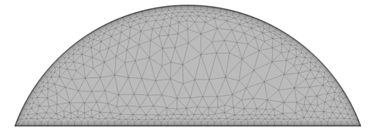
In the Model Builder window, expand the Component 1 (comp1) > Meshes > Mesh 2 > Free Triangular 1 node, then click Size 1.
2
In the Settings window for Size, locate the Element Size section.
3
From the Predefined list, choose Coarse.
Boundary Layer Properties
1
In the Model Builder window, expand the Component 1 (comp1) > Meshes > Mesh 2 > Boundary Layers 1 node, then click Boundary Layer Properties.
2
In the Settings window for Boundary Layer Properties, locate the Layers section.
3
In the Number of layers text field, type 15.
4
In the Stretching factor text field, type 1.2.
5
In the Model Builder window, right-click Mesh 2 and choose Duplicate.
Mesh 3
Size
1
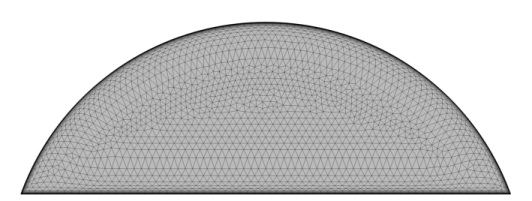
In the Model Builder window, expand the Component 1 (comp1) > Meshes > Mesh 3 node, then click Size.
2
In the Settings window for Size, locate the Element Size section.
3
From the Predefined list, choose Fine.
Size 1
1
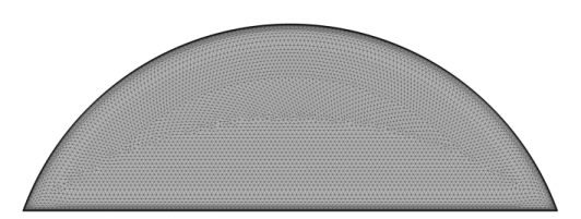
In the Model Builder window, expand the Component 1 (comp1) > Meshes > Mesh 3 > Free Triangular 1 node, then click Size 1.
2
In the Settings window for Size, locate the Element Size section.
3
From the Predefined list, choose Fine.
Boundary Layers 1
In simulations of duct flows, many iterations are required to transport the high turbulence viscosity generated by high shear near the walls to the duct center. Thus, first obtain a solution on the coarse Mesh 1, and then continue by solving on Mesh 2 and Mesh 3.
1
In the Model Builder window, expand the Component 1 (comp1) > Meshes > Mesh 3 > Boundary Layers 1 node.
Study 1
Step 1: Wall Distance Initialization, Step 2: Stationary
1
In the Model Builder window, under Study 1, Ctrl-click to select Step 1: Wall Distance Initialization and Step 2: Stationary.
2
Step 3: Wall Distance Initialization 1
1
In the Settings window for Wall Distance Initialization, click to expand the Mesh Selection section.
2
Step 4: Stationary 1
1
In the Model Builder window, click Step 4: Stationary 1.
2
In the Settings window for Stationary, click to expand the Mesh Selection section.
3
Step 3: Wall Distance Initialization 1, Step 4: Stationary 1
1
In the Model Builder window, under Study 1, Ctrl-click to select Step 3: Wall Distance Initialization 1 and Step 4: Stationary 1.
2
Step 5: Wall Distance Initialization 2
1
In the Settings window for Wall Distance Initialization, locate the Mesh Selection section.
2
Step 6: Stationary 2
1
In the Model Builder window, click Step 6: Stationary 2.
2
In the Settings window for Stationary, locate the Mesh Selection section.
3
Solution 1 (sol1)
1
In the Study toolbar, click  Show Default Solver.
2
In the Model Builder window, expand the Solution 1 (sol1) node.
3
In the Model Builder window, expand the Study 1 > Solver Configurations > Solution 1 (sol1) > Stationary Solver 2 node, then click Segregated 1.
4
In the Settings window for Segregated, locate the General section.
5
From the Termination technique list, choose Iterations or tolerance.
6
In the Number of iterations text field, type 100.
7
In the Model Builder window, expand the Study 1 > Solver Configurations > Solution 1 (sol1) > Stationary Solver 4 node, then click Segregated 1.
8
In the Settings window for Segregated, locate the General section.
9
From the Termination technique list, choose Iterations or tolerance.
10
In the Number of iterations text field, type 30.
11
In the Initial CFL number text field, type 5.
12
In the Model Builder window, expand the Study 1 > Solver Configurations > Solution 1 (sol1) > Stationary Solver 6 node, then click Segregated 1.
13
In the Settings window for Segregated, locate the General section.
14
From the Termination technique list, choose Iterations or tolerance.
15
In the Number of iterations text field, type 30.
16
In the Initial CFL number text field, type 20.
17
In the Model Builder window, click Study 1.
18
In the Settings window for Study, locate the Study Settings section.
19
Clear the Generate default plots checkbox.
20
In the Study toolbar, click  Compute.
Results
1
In the Model Builder window, click Results.
2
In the Settings window for Results, locate the Update of Results section.
3
Select the Only plot when requested checkbox.
Create datasets to be used in plots.
Surface 1
1
In the Model Builder window, expand the Results node.
2
Right-click Results > Datasets and choose Surface.
3
In the Settings window for Surface, locate the Parameterization section.
4
From the x- and y-axes list, choose xy-plane.
5
Locate the Selection section. From the Selection list, choose Central Plane.
Cut Line 2D 1
1
In the Results toolbar, click  Cut Line 2D.
2
In the Settings window for Cut Line 2D, locate the Line Data section.
3
In row Point 2, set x to 0.
4
In row Point 2, set y to h_duct.
5
Select the Additional parallel lines checkbox.
6
Click  Range.
7
In the Range dialog, type 6 in the Start text field.
8
In the Step text field, type 6.
9
In the Stop text field, type 42.
10
Click Add.
Cut Line 2D 2
1
In the Results toolbar, click  Cut Line 2D.
2
In the Settings window for Cut Line 2D, locate the Line Data section.
3
In row Point 1, set x to 5.
4
In row Point 2, set x to 5.
5
In row Point 2, set y to h_duct.
Cut Line 2D 3
1
Right-click Cut Line 2D 2 and choose Duplicate.
2
In the Settings window for Cut Line 2D, locate the Line Data section.
3
In row Point 1, set x to 15.
4
In row Point 2, set x to 15.
Cut Line 2D 4
1
Right-click Cut Line 2D 3 and choose Duplicate.
2
In the Settings window for Cut Line 2D, locate the Line Data section.
3
In row Point 1, set x to 25.
4
In row Point 2, set x to 25.
Cut Line 2D 5
1
Right-click Cut Line 2D 4 and choose Duplicate.
2
In the Settings window for Cut Line 2D, locate the Line Data section.
3
In row Point 1, set x to 35.
4
In row Point 2, set x to 35.
Evaluate control quantities on all the meshes.
Evaluation Group 1
In the Results toolbar, click  Evaluation Group.
Streamwise Friction Coefficient
1
Right-click Evaluation Group 1 and choose Average > Surface Average.
2
In the Settings window for Surface Average, type Streamwise Friction Coefficient in the Label text field.
3
Locate the Selection section. From the Selection list, choose Walls.
4
Locate the Expressions section. In the table, enter the following settings:
Cross-Stream Friction Coefficient
1
Right-click Streamwise Friction Coefficient and choose Duplicate.
2
In the Settings window for Surface Average, type Cross-Stream Friction Coefficient in the Label text field.
3
Locate the Expressions section. In the table, enter the following settings:
4
In the Evaluation Group 1 toolbar, click  Evaluate.
The results presented in the plots are from the solution obtained on Mesh 3.
Surface Streamlines
1
In the Results toolbar, click  2D Plot Group.
2
In the Settings window for 2D Plot Group, type Surface Streamlines in the Label text field.
3
Click to expand the Title section. From the Title type list, choose Manual.
4
In the Title text area, type Streamline surface and Arrow surface of the Secondary velocity field.
5
Click to expand the Plot Array section. Select the Enable checkbox.
6
From the Array axis list, choose y.
7
In the Relative padding text field, type -2.25.
Streamline 1
1
Right-click Surface Streamlines and choose Streamline.
2
In the Settings window for Streamline, locate the Streamline Positioning section.
3
From the Positioning list, choose Uniform density.
4
In the Density level text field, type 10.8.
Color Expression 1
1
Right-click Streamline 1 and choose Color Expression.
2
In the Settings window for Color Expression, locate the Expression section.
3
In the Expression text field, type sqrt(u^2+v^2)/Ub.
4
Locate the Coloring and Style section. From the Color table list, choose Ranitomeya.
Check that the results on Mesh 1 and even on Mesh 2 provide streamlines that are not as smooth as those obtained using Mesh 3.
Arrow Surface 1
1
In the Model Builder window, right-click Surface Streamlines and choose Arrow Surface.
2
In the Settings window for Arrow Surface, locate the Arrow Positioning section.
3
Find the x grid points subsection. In the Points text field, type 30.
4
Find the y grid points subsection. In the Points text field, type 30.
5
Locate the Coloring and Style section.
6
Select the Scale factor checkbox. In the associated text field, type 250.
7
From the Color list, choose Black.
8
In the Surface Streamlines toolbar, click  Plot.
9
Click the  Zoom Extents button in the Graphics toolbar.
Streamwise Velocity: Average Friction Scaling
1
In the Results toolbar, click  1D Plot Group.
2
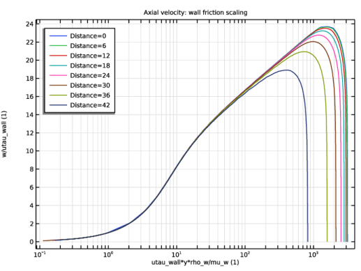
In the Settings window for 1D Plot Group, type Streamwise Velocity: Average Friction Scaling in the Label text field.
3
Click to expand the Title section. From the Title type list, choose Manual.
4
In the Title text area, type Axial velocity: average friction scaling.
5
Locate the Data section. From the Dataset list, choose Cut Line 2D 1.
6
Locate the Legend section. From the Position list, choose Upper left.
Line Graph 1
1
Right-click Streamwise Velocity: Average Friction Scaling and choose Line Graph.
2
In the Settings window for Line Graph, locate the y-Axis Data section.
3
In the Expression text field, type w/utau_av.
4
Locate the x-Axis Data section. From the Parameter list, choose Expression.
5
In the Expression text field, type utau_av*y*rho_w/mu_w.
6
Click the  x-Axis Log Scale button in the Graphics toolbar.
7
Click to expand the Coloring and Style section. From the Color cycle list, choose Long.
8
Click to expand the Legends section. Select the Show legends checkbox.
Streamwise Velocity: Wall Friction Scaling
1
In the Model Builder window, right-click Streamwise Velocity: Average Friction Scaling and choose Duplicate.
2
In the Settings window for 1D Plot Group, type Streamwise Velocity: Wall Friction Scaling in the Label text field.
3
Locate the Title section. In the Title text area, type Axial velocity: wall friction scaling.
Line Graph 1
1
In the Model Builder window, expand the Streamwise Velocity: Wall Friction Scaling node, then click Line Graph 1.
2
In the Settings window for Line Graph, locate the y-Axis Data section.
3
In the Expression text field, type w/utau_wall.
4
Locate the x-Axis Data section. In the Expression text field, type utau_wall*y*rho_w/mu_w.
Secondary Flow: u-Component
1
In the Model Builder window, right-click Streamwise Velocity: Average Friction Scaling and choose Duplicate.
2
In the Settings window for 1D Plot Group, type Secondary Flow: u-Component in the Label text field.
3
Locate the Title section. In the Title text area, type Velocity x-component.
4
Locate the Legend section. From the Position list, choose Upper right.
Line Graph 1
1
In the Model Builder window, expand the Secondary Flow: u-Component node, then click Line Graph 1.
2
In the Settings window for Line Graph, locate the y-Axis Data section.
3
In the Expression text field, type u.
4
Locate the x-Axis Data section. In the Expression text field, type y.
5
Click the  x-Axis Log Scale button in the Graphics toolbar.
Secondary Flow: v-Component
1
In the Model Builder window, right-click Secondary Flow: u-Component and choose Duplicate.
2
In the Settings window for 1D Plot Group, type Secondary Flow: v-Component in the Label text field.
3
Locate the Title section. In the Title text area, type Velocity y-component.
Line Graph 1
1
In the Model Builder window, expand the Secondary Flow: v-Component node, then click Line Graph 1.
2
In the Settings window for Line Graph, locate the y-Axis Data section.
3
In the Expression text field, type v.
Streamwise Vorticity Contours and Plots
1
In the Results toolbar, click  2D Plot Group.
Illustrate the streamwise vorticity due to the secondary flow.
2
In the Settings window for 2D Plot Group, type Streamwise Vorticity Contours and Plots in the Label text field.
3
Locate the Title section. From the Title type list, choose Manual.
4
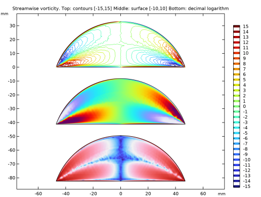
In the Title text area, type Streamwise vorticity. Top: contours [-15,15] Middle: surface [-10,10] Bottom: decimal logarithm.
5
Locate the Plot Array section. Select the Enable checkbox.
6
From the Array axis list, choose y.
7
In the Relative padding text field, type -2.25.
Contour 1
1
Right-click Streamwise Vorticity Contours and Plots and choose Contour.
2
In the Settings window for Contour, locate the Expression section.
3
In the Expression text field, type max(min(15,spf.vorticityz),-15).
4
Locate the Levels section. From the Entry method list, choose Levels.
5
In the Levels text field, type range(-15,1,15).
Surface 1
1
In the Model Builder window, right-click Streamwise Vorticity Contours and Plots and choose Surface.
2
In the Settings window for Surface, locate the Expression section.
3
In the Expression text field, type max(min(10,spf.vorticityz),-10).
4
Locate the Coloring and Style section. From the Color table list, choose Prism.
5
Clear the Color legend checkbox.
Surface 2
1
Right-click Surface 1 and choose Duplicate.
2
In the Settings window for Surface, locate the Expression section.
3
In the Expression text field, type log10(spf.vorticityz).
4
Locate the Coloring and Style section. From the Color table list, choose Wave.
5
In the Streamwise Vorticity Contours and Plots toolbar, click  Plot.
6
Click the  Zoom Extents button in the Graphics toolbar.
Plot the streamlines in a 3D view. Significant compression in the streamwise direction is needed for good visualization of the secondary flow.
Secondary Flow in 3D
1
In the Results toolbar, click  3D Plot Group.
2
In the Settings window for 3D Plot Group, type Secondary Flow in 3D in the Label text field.
3
Click to expand the Title section. From the Title type list, choose Manual.
4
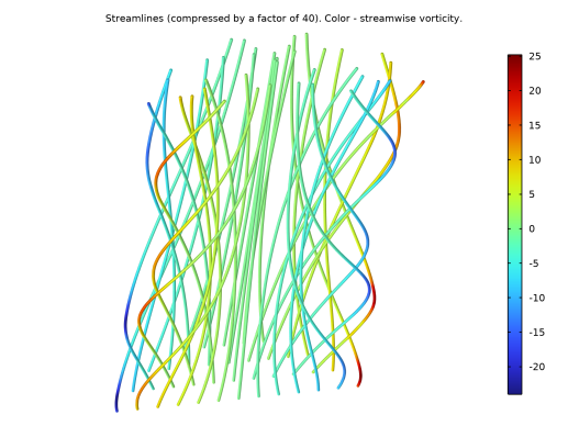
In the Title text area, type Streamlines (compressed by a factor of 40). Color - streamwise vorticity..
5
Locate the Plot Settings section. Clear the Plot dataset edges checkbox.
6
From the View list, choose New view.
7
In the Secondary Flow in 3D toolbar, click  Plot.
Streamline 1
1
Right-click Secondary Flow in 3D and choose Streamline.
2
In the Settings window for Streamline, locate the Expression section.
3
In the z-component text field, type w/1000.
4
Locate the Streamline Positioning section. In the Number text field, type 40.
5
6
Locate the Coloring and Style section. Find the Line style subsection. From the Type list, choose Tube.
7
Select the Radius scale factor checkbox. In the associated text field, type 0.5.
Color Expression 1
1
Right-click Streamline 1 and choose Color Expression.
2
In the Settings window for Color Expression, locate the Expression section.
3
In the Expression text field, type spf.vorticityz.
Transformation 1
1
In the Model Builder window, right-click Streamline 1 and choose Transformation.
2
In the Settings window for Transformation, locate the Transformation section.
3
Select the Scale checkbox.
4
In the z text field, type 25.
5
In the Secondary Flow in 3D toolbar, click  Plot.
Axial and Secondary (u) Velocity, muT/mu
1
In the Results toolbar, click  2D Plot Group.
2
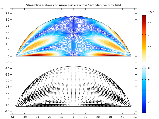
In the Settings window for 2D Plot Group, type Axial and Secondary (u) Velocity, muT/mu in the Label text field.
3
Locate the Title section. From the Title type list, choose Manual.
4
In the Title text area, type Top: axial velocity, middle: secondary velocity (u), bottom: muT/mu.
5
Locate the Plot Array section. Select the Enable checkbox.
6
From the Array axis list, choose y.
7
In the Relative padding text field, type 0.25.
Surface 1
1
Right-click Axial and Secondary (u) Velocity, muT/mu and choose Surface.
2
In the Settings window for Surface, locate the Expression section.
3
In the Expression text field, type spf.muT/spf.mu.
4
Locate the Coloring and Style section. From the Color table list, choose Thermal.
5
Clear the Color legend checkbox.
Surface 2
1
In the Model Builder window, right-click Axial and Secondary (u) Velocity, muT/mu and choose Surface.
2
In the Settings window for Surface, locate the Expression section.
3
In the Expression text field, type sqrt(u^2+v^2)/Ub.
4
Locate the Coloring and Style section. From the Color table list, choose Ranitomeya.
Surface 3
1
Right-click Axial and Secondary (u) Velocity, muT/mu and choose Surface.
2
In the Settings window for Surface, locate the Expression section.
3
In the Expression text field, type w/Ub.
4
Locate the Coloring and Style section. From the Color table list, choose Viridis.
5
Clear the Color legend checkbox.
6
In the Axial and Secondary (u) Velocity, muT/mu toolbar, click  Plot.
7
Click the  Zoom Extents button in the Graphics toolbar.
uu, vv, uu-vv
1
In the Results toolbar, click  2D Plot Group.
2
In the Settings window for 2D Plot Group, type uu, vv, uu-vv in the Label text field.
3
Locate the Title section. From the Title type list, choose Manual.
4
In the Title text area, type Top: uu, Middle: vv, Bottom: uu-vv.
5
Locate the Plot Array section. Select the Enable checkbox.
6
From the Array axis list, choose y.
7
In the Relative padding text field, type 0.25.
Surface 1
1
Right-click uu, vv, uu-vv and choose Surface.
2
In the Settings window for Surface, locate the Expression section.
3
In the Expression text field, type uu-vv.
4
Locate the Coloring and Style section. From the Color table list, choose Ranitomeya.
Surface 2
1
Right-click Surface 1 and choose Duplicate.
2
In the Settings window for Surface, locate the Expression section.
3
In the Expression text field, type vv.
4
Click to expand the Inherit Style section. From the Plot list, choose Surface 1.
Surface 3
1
Right-click Surface 2 and choose Duplicate.
2
In the Settings window for Surface, locate the Expression section.
3
In the Expression text field, type uu.
4
In the uu, vv, uu-vv toolbar, click  Plot.
5
Click the  Zoom Extents button in the Graphics toolbar.
uv, uw, vw
1
In the Results toolbar, click  2D Plot Group.
2
In the Settings window for 2D Plot Group, type uv, uw, vw in the Label text field.
3
Locate the Title section. From the Title type list, choose Manual.
4
In the Title text area, type Top: uv, Middle: uw, Bottom: vw.
5
Locate the Plot Array section. Select the Enable checkbox.
6
From the Array axis list, choose y.
7
In the Relative padding text field, type 0.25.
Surface 1
1
Right-click uv, uw, vw and choose Surface.
2
In the Settings window for Surface, locate the Expression section.
3
In the Expression text field, type vw.
4
Locate the Coloring and Style section. From the Color table list, choose Ranitomeya.
Surface 2
1
Right-click Surface 1 and choose Duplicate.
2
In the Settings window for Surface, locate the Expression section.
3
In the Expression text field, type uw.
4
Locate the Inherit Style section. From the Plot list, choose Surface 1.
Surface 3
1
Right-click Surface 2 and choose Duplicate.
2
In the Settings window for Surface, locate the Expression section.
3
In the Expression text field, type uv.
4
In the uv, uw, vw toolbar, click  Plot.
5
Click the  Zoom Extents button in the Graphics toolbar.
ww and Turbulence Kinetic Energy
1
In the Results toolbar, click  2D Plot Group.
2
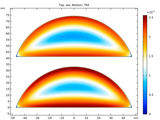
In the Settings window for 2D Plot Group, type ww and Turbulence Kinetic Energy in the Label text field.
3
Locate the Title section. From the Title type list, choose Manual.
4
In the Title text area, type Top: ww, Bottom: TKE.
5
Locate the Plot Array section. Select the Enable checkbox.
6
From the Array axis list, choose y.
7
In the Relative padding text field, type 0.25.
Surface 1
1
Right-click ww and Turbulence Kinetic Energy and choose Surface.
2
In the Settings window for Surface, locate the Expression section.
3
In the Expression text field, type spf.tke.
4
Locate the Coloring and Style section. From the Color table list, choose Ranitomeya.
Surface 2
1
Right-click Surface 1 and choose Duplicate.
2
In the Settings window for Surface, locate the Expression section.
3
In the Expression text field, type ww.
4
Locate the Inherit Style section. From the Plot list, choose Surface 1.
5
Click the  Zoom Extents button in the Graphics toolbar.