PDF

Self-Lubricating Journal Bearing
Introduction
A self-lubricating journal bearing typically has a porous bush which is press-fitted to the bearing, such that, the bush’s inner surface and the rotating journal maintain a small, lubricant-filled clearance. The porous bush, usually made of sintered metal powder, is impregnated with the lubricant. During operation, the bush acts as a reservoir and redistributes the lubricant in the clearance.
Inside the porous bush, the lubricant is permitted to flow along axial, radial and circumferential directions. When the journal is loaded, it is no longer concentric with the bush. This eccentricity creates a zone of high lubricant pressure in the region of reducing clearance and a zone of low lubricant pressure in the region of increasing clearance. The lubricant is supplied into the clearance from the pores in the low pressure zone and simultaneously squeezed out of the high pressure zone into the porous bush, thus facilitating the act of self-lubrication.
These bearings are generally employed in applications operating under high rotational speed and low load-carrying requirements. They are most useful in situations where frequent maintenance and lubrication of the bearing is not feasible.
Model Definition
This model simulates a journal bearing operating in the hydrodynamic lubrication regime. In this regime, the lubricant is assumed to fill the entire clearance between the rotating journal and the bush, thereby generating high- and low-pressure zones, of which the former helps to support the external load. The phenomenon of cavitation, which can typically occur in the low-pressure zone, is ignored in the model.
The migration of lubricant in the porous bush is modeled using Darcy’s law. The flow of the thin film of lubricant in the clearance is modeled using the Reynolds equation. At the interface between the porous and thin-film flow regions, the boundary layer developed is modeled using the Beavers–Joseph condition, which proposes an interface slip velocity for the clear fluid (thin-film fluid in the present example) that is proportional to the normal exterior velocity gradient. For details, see Ref. 1.
The dimensionless quantities of interest, reported in Ref. 1, are
(1)
Here, s is the dimensionless slip parameter, Φ is the permeability of the porous bush, α is the Beavers–Joseph slip coefficient, C is the concentric clearance between the journal and the bush, Ψ is the dimensionless permeability parameter, and H is the radial thickness of the bush. The thickness of the thin film of fluid in the clearance, ht, is determined by the eccentricity, ε, as ht = C(1 + εcosθ), where, θ = atan(y/x) is the angular position in the xy-plane.
The model solves for the stationary solution of the flow field in the porous domain and the clearance for the parameter values , , and . It compares the numerical solution with those obtained from the analytic expressions in Ref. 1 for the short-bearing approximation, where the radius is much larger than the bearing length. Further, the flow field is visualized for a typical bearing without the short-bearing assumption.
Geometry
The geometry represents the porous bush as a cylindrical annulus, wherein the clearance is represented by the bush’s inner surface, as shown in Figure 1.
Figure 1: Computational domain of the porous bush. The clearance is represented by the inner surface of the cylinder.
The journal and the bearing are not represented in the geometry of the model, but their influence is taken into consideration in the form of boundary conditions. The bush has an inner radius, R, and length along the axis, L = 5H. For the short-bearing assumption, R = 20L; otherwise, R = L. For all simulations, the concentric clearance, C = 105 m.
Physics Interface Settings
The lubricant density is ρ = kg·m3 and the dynamic viscosity μ = Pa·s. The journal’s tangential velocity is U = m/s. The Thin-Film Flow interface solves the Reynolds equation. The fluid-film thickness in the clearance is specified as the height of the wall, while the tangential velocity is specified at the base. The two ends of the bearing are assumed to be exposed to ambient conditions. Hence, a zero-pressure boundary condition is applicable. Meanwhile, a no-penetration condition is suitable at the bush surface that is in contact with the nonporous bearing to model the press-fit. For both interfaces, the reference pressure, pref = 0. Also, a zero-pressure initial condition is applied. The Thin-Film and Porous Media Flow multiphysics coupling with a Beavers–Joseph slip condition couples the interfaces.
Meshing
A structured mesh composed of hexahedral elements is constructed with 200, 5, and 15 elements in the circumferential, radial, and axial directions, respectively, as shown in Figure 2.
Figure 2: A structured, hexahedral mesh for the cylindrical geometry.
Results and Discussion
The load-carrying capacity is the main quantity of interest for postprocessing the solution. A dimensionless form of the load-carrying capacity, Wnd, can be calculated from the computed pressure as
(2)
Here, pfilm is the thin-film pressure. Negative pressures are ignored according to Ocvirk’s approximations; see Ref. 1. The analytic expression for the nondimensional load-carrying capacity, Wnd,ana, obtained from Ref. 1, is given by
(3)
where the dimensionless pressure, pnd, is given by
(4)
Here,
(5)
(6)
(7)
(8)
Figure 3 shows a plot of the nondimensional load-carrying capacity as a function of ε for various values of Ψ. The numeric values match well with the analytic curves.
Figure 3: The dimensionless load-carrying capacity as a function of eccentricity for different values of the permeability parameter. Here, s = 0.25.
Dotted lines show the load capacity with no slip at the interface. Load capacity generally increases with increased eccentricity for all values of Ψ. Accounting for the slip results in a reduction in the load capacity for low values of eccentricity. This is true up to a certain critical value of transition of ε that depends on Ψ. Thereafter, the trend reverses for larger values of eccentricity. Also, for small values of Ψ, the load capacity is large, indicating that the load capacity deteriorates with increases in the permeability of the porous bush.
Figure 4 shows the plot of the nondimensional load-carrying capacity as a function of Ψ for various values of ε. The numeric values match well with the analytic curves.
Figure 4: The dimensionless load-carrying capacity as a function of the permeability parameter for different values of eccentricity. Here, s = 0.25.
In general, the load capacity decreases with increases in the permeability parameter, where higher values of eccentricity support higher load values. Here, the dotted lines show the load capacity with no slip at the interface. Accounting for the slip velocity, the load capacities are smaller than those with no-slip condition up to a certain critical value of Ψ, after which the trend is observed to reverse. Moreover, the critical value of transition for Ψ decreases with increased eccentricity.
Figure 5 and Figure 6 show a similar behavior to that in Figure 3 and Figure 4, respectively, thus indicating that the effect of an increase in the slip coefficient value is not significant.
Figure 5: The dimensionless load carrying capacity as a function of eccentricity for different values of the permeability parameter. Here, s = 0.5.
Figure 7 shows a polar plot of the attitude angle, versus the eccentricity for various values of the permeability parameter. Again, the dotted lines show the load capacity with no slip at the interface. The attitude angle is the angle formed by the line joining the centers of the journal and the bearing with the load line. It is computed from the numerical solution as
(9)
The analytic expression for the attitude angle, obtained from Ref. 1, is given by
(10)
The attitude angle generally decreases with increases in the eccentricity and decreases in the permeability parameter. Compared to the case of no slip at the interface, a slip condition generally produces a lower attitude angle. The exceptional case is for the low value of Ψ = 0.001, where for lower values of eccentricity the attitude angle is larger for the slip condition as compared to that for the no-slip condition.
Figure 6: The dimensionless load carrying capacity as a function of the permeability parameter for different values of eccentricity. Here, s = 0.5.
Figure 8 shows the steady-state flow patterns in a typical self-lubricating bearing. The pressure contours show the development of differential pressure zones. The streamlines show the flow of the lubricant from high pressure zone to the low pressure zone and also the loss of lubricant at the ends of the bearing which are exposed to ambient conditions.
Figure 7: Polar plot of the attitude angle vs. eccentricity for different values of the permeability parameter.
Figure 8: Streamlines showing the flow of lubricant in the porous bush of a self-lubricating journal bearing. Also shown are the contours of pressure and the variation of thickness of the thin film of fluid in the gap between the bush and the journal.
Reference
1. J. Prakash and S.K. Vij, “Analysis of Narrow Porous Journal Bearing Using Beavers-Joseph Criterion of Velocity Slip,” J. Appl. Mech., vol. 41, no. 2, pp. 348–354, 1974.
Application Library path: CFD_Module/Verification_Examples/self_lubricating_bearing
Modeling Instructions
From the File menu, choose New.
New
In the New window, click  Model Wizard.
Model Wizard
1
In the Model Wizard window, click  3D.
2
In the Select Physics tree, select Fluid Flow > Porous Media and Subsurface Flow > Thin-Film and Porous Media Flow.
3
Click Add.
4
Click  Study.
5
In the Select Study tree, select General Studies > Stationary.
6
Global Definitions
Load parameters and variables from file.
Parameters 1
1
In the Model Builder window, under Global Definitions click Parameters 1.
2
In the Settings window for Parameters, locate the Parameters section.
3
Click  Load from File.
4
Definitions
Variables 1
1
In the Model Builder window, under Component 1 (comp1) right-click Definitions and choose Variables.
2
In the Settings window for Variables, locate the Variables section.
3
Click  Load from File.
4
Analytic 1 (an1)
Create help functions for the analytic solution.
1
In the Definitions toolbar, click  Analytic.
2
In the Settings window for Analytic, type beta_n in the Function name text field.
3
Locate the Definition section. In the Expression text field, type 2*n-1.
4
In the Arguments text field, type n.
5
Locate the Plot Parameters section. In the table, enter the following settings:
Analytic 2 (an2)
1
In the Definitions toolbar, click  Analytic.
2
In the Settings window for Analytic, type g_n in the Function name text field.
3
Locate the Definition section. In the Expression text field, type sin(theta)*(2*s^2+2*s*(1+ep*cos(theta))+(1+ep*cos(theta))^2)/((s+1+ep*cos(theta))*(((6*(alpha^2)*(s^2)+4*s*(1+ep*cos(theta))+(1+ep*cos(theta))^2)*(1+ep*cos(theta))^2)+(12*Psi*(s+1+ep*cos(theta))*tanh(pi*beta_n(n)*H/L)/(pi*beta_n(n)*H/L)))).
4
In the Arguments text field, type ep, n, Psi, s, theta.
5
Locate the Plot Parameters section. In the table, enter the following settings:
Analytic 3 (an3)
1
In the Definitions toolbar, click  Analytic.
2
In the Settings window for Analytic, type pbar_summand in the Function name text field.
3
Locate the Definition section. In the Expression text field, type (-1)^(n+1)*ep*g_n(ep,n,Psi,s,theta)*cos(pi*beta_n(n)*z/L)/(2*n-1)^3.
4
In the Arguments text field, type ep, n, Psi, s, theta, z.
5
Locate the Plot Parameters section. In the table, enter the following settings:
Geometry 1
Cylinder 1 (cyl1)
1
In the Geometry toolbar, click  Cylinder.
2
In the Settings window for Cylinder, locate the Object Type section.
3
From the Type list, choose Surface.
4
Locate the Size and Shape section. In the Radius text field, type R+H.
5
In the Height text field, type L.
6
Locate the Position section. In the z text field, type -L/2.
7
Click to expand the Layers section. In the table, enter the following settings:
Form Union (fin)
In the Geometry toolbar, click  Build All.
Thin-Film Flow (tff)
1
In the Model Builder window, under Component 1 (comp1) click Thin-Film Flow (tff).
2
In the Settings window for Thin-Film Flow, locate the Boundary Selection section.
3
Click  Clear Selection.
4
Click  Paste Selection.
5
In the Paste Selection dialog, type 8, 9, 14, 16 in the Selection text field.
6
7
In the Settings window for Thin-Film Flow, locate the Reference Pressure section.
8
In the pref text field, type 0.
Fluid-Film Properties 1
1
In the Model Builder window, under Component 1 (comp1) > Thin-Film Flow (tff) click Fluid-Film Properties 1.
2
In the Settings window for Fluid-Film Properties, locate the Wall Properties section.
3
In the hw1 text field, type h_f.
4
Locate the Base Properties section. From the vb list, choose User defined. Specify the vector as
5
Locate the Fluid Properties section. From the μ list, choose User defined. In the associated text field, type mu.
6
From the ρ list, choose User defined. In the associated text field, type rho.
Darcy’s Law (dl)
1
In the Model Builder window, under Component 1 (comp1) click Darcy’s Law (dl).
2
In the Settings window for Darcy’s Law, locate the Physical Model section.
3
In the pref text field, type 0.
Fluid 1
1
In the Model Builder window, under Component 1 (comp1) > Darcy’s Law (dl) > Porous Medium 1 click Fluid 1.
2
In the Settings window for Fluid, locate the Fluid Properties section.
3
From the ρ list, choose User defined. In the associated text field, type rho.
4
From the μ list, choose User defined. In the associated text field, type mu.
Porous Matrix 1
1
In the Model Builder window, click Porous Matrix 1.
2
In the Settings window for Porous Matrix, locate the Matrix Properties section.
3
From the κ list, choose User defined. In the associated text field, type Phi.
4
From the εp list, choose User defined.
Pressure 1
1
In the Physics toolbar, click  Boundaries and choose Pressure.
2
In the Settings window for Pressure, locate the Boundary Selection section.
3
Click  Paste Selection.
4
In the Paste Selection dialog, type 4-7, 12, 13, 17, 18 in the Selection text field.
5
Multiphysics
Thin-Film and Porous Media Flow 1 (tfpf1)
1
In the Model Builder window, under Component 1 (comp1) > Multiphysics click Thin-Film and Porous Media Flow 1 (tfpf1).
2
In the Settings window for Thin-Film and Porous Media Flow, locate the Coupling section.
3
From the Coupling type list, choose Beavers–Joseph slip condition.
4
In the αBJ,w text field, type alpha.
5
In the αBJ,b text field, type alpha.
Mesh 1
Create a structured mesh.
1
In the Model Builder window, under Component 1 (comp1) click Mesh 1.
2
In the Settings window for Mesh, locate the Sequence Type section.
3
From the list, choose User-controlled mesh.
Edge 1
1
In the Mesh toolbar, click  More Generators and choose Edge.
2
In the Settings window for Edge, locate the Edge Selection section.
3
Click  Paste Selection.
4
In the Paste Selection dialog, type 3, 4, 9, 10, 15, 19, 23, 27 in the Selection text field.
5
Distribution 1
1
Right-click Edge 1 and choose Distribution.
2
In the Settings window for Distribution, locate the Distribution section.
3
In the Number of elements text field, type 50.
4
Select the Equidistant checkbox.
Mapped 1
1
In the Mesh toolbar, click  More Generators and choose Mapped.
2
In the Settings window for Mapped, locate the Boundary Selection section.
3
Click  Paste Selection.
4
In the Paste Selection dialog, type 4, 5, 12, 17 in the Selection text field.
5
Distribution 1
1
Right-click Mapped 1 and choose Distribution.
2
In the Settings window for Distribution, locate the Edge Selection section.
3
Click  Paste Selection.
4
In the Paste Selection dialog, type 2, 14, 22, 30 in the Selection text field.
5
Swept 1
In the Mesh toolbar, click  Swept.
Distribution 1
1
Right-click Swept 1 and choose Distribution.
2
In the Settings window for Distribution, locate the Distribution section.
3
In the Number of elements text field, type 15.
Free Tetrahedral 1
1
In the Model Builder window, under Component 1 (comp1) > Mesh 1 right-click Free Tetrahedral 1 and choose Disable.
2
Right-click Mesh 1 and choose Build All.
Definitions
Add integration operators required later for solution postprocessing.
Integration 1 (intop1)
1
In the Definitions toolbar, click  Nonlocal Couplings and choose Integration.
2
In the Settings window for Integration, locate the Source Selection section.
3
From the Geometric entity level list, choose Boundary.
4
Click  Paste Selection.
5
In the Paste Selection dialog, type 9, 16 in the Selection text field.
6
Integration 2 (intop2)
1
In the Definitions toolbar, click  Nonlocal Couplings and choose Integration.
2
In the Settings window for Integration, locate the Source Selection section.
3
From the Geometric entity level list, choose Boundary.
4
Click  Paste Selection.
5
In the Paste Selection dialog, type 8, 9, 14, 16 in the Selection text field.
6
Global Definitions
Solve the Stationary study step for different values of parameters s, Phi and ep. The short-bearing assumption is applicable.
Parameters 1
1
In the Model Builder window, under Global Definitions click Parameters 1.
2
In the Settings window for Parameters, locate the Parameters section.
3
Study 1
Parametric Sweep
1
In the Study toolbar, click  Parametric Sweep.
2
In the Settings window for Parametric Sweep, locate the Study Settings section.
3
4
5
6
7
8
9
From the Sweep type list, choose All combinations.
10
In the Model Builder window, click Study 1.
11
In the Settings window for Study, locate the Study Settings section.
12
Clear the Generate default plots checkbox.
13
In the Study toolbar, click  Compute.
Global Definitions
Solve the Stationary study step without the short-bearing assumption
Parameters 1
1
In the Model Builder window, under Global Definitions click Parameters 1.
2
In the Settings window for Parameters, locate the Parameters section.
3
Add Study
1
In the Home toolbar, click  Add Study to open the Add Study window.
2
Go to the Add Study window.
3
Find the Studies subsection. In the Select Study tree, select General Studies > Stationary.
4
Click the Add Study button in the window toolbar.
5
In the Home toolbar, click  Add Study to close the Add Study window.
Study 2
1
In the Settings window for Study, locate the Study Settings section.
2
Clear the Generate default plots checkbox.
3
In the Study toolbar, click  Compute.
Results
1
In the Model Builder window, click Results.
2
In the Settings window for Results, locate the Update of Results section.
3
Select the Only plot when requested checkbox.
Grid 1D 1
Create datasets to plot the analytic expressions of the solution.
1
In the Model Builder window, expand the Results node.
2
Right-click Results > Datasets and choose More Datasets > Grid 1D.
3
In the Settings window for Grid 1D, locate the Data section.
4
From the Source list, choose Function.
5
From the Function list, choose All.
6
Locate the Parameter Bounds section. In the Name text field, type ep.
Grid 1D 2
1
Right-click Grid 1D 1 and choose Duplicate.
2
In the Settings window for Grid 1D, locate the Parameter Bounds section.
3
In the Name text field, type Psi.
4
In the Minimum text field, type 0.001.
Global Evaluation 1
Derive numeric values of the dimensionless load and attitude angle for different parameter combinations.
1
In the Results toolbar, click  Global Evaluation.
2
In the Settings window for Global Evaluation, locate the Data section.
3
From the Dataset list, choose Study 1/Parametric Solutions 1 (sol2).
4
From the Parameter selection (s) list, choose From list.
5
In the Parameter values (s) list box, select 0.25.
6
From the Parameter selection (Psi) list, choose From list.
7
In the Parameter values (Psi) list box, select 1.
8
Locate the Expressions section. In the table, enter the following settings:
Global Evaluation 2
1
Right-click Global Evaluation 1 and choose Duplicate.
2
In the Settings window for Global Evaluation, locate the Data section.
3
In the Parameter values (Psi) list box, select 0.1.
Global Evaluation 3
1
Right-click Global Evaluation 2 and choose Duplicate.
2
In the Settings window for Global Evaluation, locate the Data section.
3
In the Parameter values (Psi) list box, select 0.01.
Global Evaluation 4
1
Right-click Global Evaluation 3 and choose Duplicate.
2
In the Settings window for Global Evaluation, locate the Data section.
3
In the Parameter values (Psi) list box, select 0.001.
Global Evaluation 5
1
In the Results toolbar, click  Global Evaluation.
2
In the Settings window for Global Evaluation, locate the Data section.
3
From the Dataset list, choose Study 1/Parametric Solutions 1 (sol2).
4
From the Parameter selection (s) list, choose From list.
5
In the Parameter values (s) list box, select 0.25.
6
From the Parameter selection (ep) list, choose From list.
7
In the Parameter values (ep) list box, select 0.1.
8
Locate the Expressions section. In the table, enter the following settings:
Global Evaluation 6
1
Right-click Global Evaluation 5 and choose Duplicate.
2
In the Settings window for Global Evaluation, locate the Data section.
3
In the Parameter values (ep) list box, select 0.3.
Global Evaluation 7
1
Right-click Global Evaluation 6 and choose Duplicate.
2
In the Settings window for Global Evaluation, locate the Data section.
3
In the Parameter values (ep) list box, select 0.5.
Global Evaluation 8
1
Right-click Global Evaluation 7 and choose Duplicate.
2
In the Settings window for Global Evaluation, locate the Data section.
3
In the Parameter values (ep) list box, select 0.7.
Global Evaluation 9
1
Right-click Global Evaluation 8 and choose Duplicate.
2
In the Settings window for Global Evaluation, locate the Data section.
3
In the Parameter values (ep) list box, select 0.9.
Global Evaluation 10
1
In the Results toolbar, click  Global Evaluation.
2
In the Settings window for Global Evaluation, locate the Data section.
3
From the Dataset list, choose Study 1/Parametric Solutions 1 (sol2).
4
From the Parameter selection (s) list, choose From list.
5
In the Parameter values (s) list box, select 0.5.
6
From the Parameter selection (Psi) list, choose From list.
7
In the Parameter values (Psi) list box, select 1.
8
Locate the Expressions section. In the table, enter the following settings:
Global Evaluation 11
1
Right-click Global Evaluation 10 and choose Duplicate.
2
In the Settings window for Global Evaluation, locate the Data section.
3
In the Parameter values (Psi) list box, select 0.1.
Global Evaluation 12
1
Right-click Global Evaluation 11 and choose Duplicate.
2
In the Settings window for Global Evaluation, locate the Data section.
3
In the Parameter values (Psi) list box, select 0.01.
Global Evaluation 13
1
Right-click Global Evaluation 12 and choose Duplicate.
2
In the Settings window for Global Evaluation, locate the Data section.
3
In the Parameter values (Psi) list box, select 0.001.
Global Evaluation 14
1
In the Results toolbar, click  Global Evaluation.
2
In the Settings window for Global Evaluation, locate the Data section.
3
From the Dataset list, choose Study 1/Parametric Solutions 1 (sol2).
4
From the Parameter selection (s) list, choose From list.
5
In the Parameter values (s) list box, select 0.5.
6
From the Parameter selection (ep) list, choose From list.
7
In the Parameter values (ep) list box, select 0.1.
8
Locate the Expressions section. In the table, enter the following settings:
Global Evaluation 15
1
Right-click Global Evaluation 14 and choose Duplicate.
2
In the Settings window for Global Evaluation, locate the Data section.
3
In the Parameter values (ep) list box, select 0.3.
Global Evaluation 16
1
Right-click Global Evaluation 15 and choose Duplicate.
2
In the Settings window for Global Evaluation, locate the Data section.
3
In the Parameter values (ep) list box, select 0.5.
Global Evaluation 17
1
Right-click Global Evaluation 16 and choose Duplicate.
2
In the Settings window for Global Evaluation, locate the Data section.
3
In the Parameter values (ep) list box, select 0.7.
Global Evaluation 18
1
Right-click Global Evaluation 17 and choose Duplicate.
2
In the Settings window for Global Evaluation, locate the Data section.
3
In the Parameter values (ep) list box, select 0.9.
4
In the Results toolbar, click  Evaluate and choose Evaluate All.
Dimensionless Load vs. ep: s=0.25
1
In the Results toolbar, click  1D Plot Group.
2
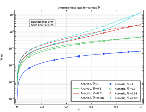
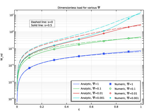
In the Settings window for 1D Plot Group, type Dimensionless Load vs. ep: s=0.25 in the Label text field.
3
Locate the Data section. From the Dataset list, choose None.
4
Click to expand the Title section. From the Title type list, choose Manual.
5
In the Title text area, type Dimensionless load for various \Psi.
6
Locate the Plot Settings section.
7
Select the x-axis label checkbox. In the associated text field, type \epsilon.
8
Select the y-axis label checkbox. In the associated text field, type W_nd.
9
Locate the Axis section. Select the y-axis log scale checkbox.
10
Locate the Legend section. From the Position list, choose Lower right.
11
In the Number of columns text field, type 2.
12
In the Maximum relative width text field, type 1.
Function 1
1
In the Dimensionless Load vs. ep: s=0.25 toolbar, click  More Plots and choose Function.
2
In the Settings window for Function, locate the Data section.
3
From the Dataset list, choose Grid 1D 1.
4
Locate the y-Axis Data section. In the Expression text field, type sqrt((integrate(integrate((24/pi^3)*sum(pbar_summand(ep,n,1,0.25,theta,z),n,1,n_upper_lim)*cos(theta),theta,0,pi),z,-L/2,L/2))^2+(integrate(integrate((24/pi^3)*sum(pbar_summand(ep,n,1,0.25,theta,z),n,1,n_upper_lim)*sin(theta),theta,0,pi),z,-L/2,L/2))^2)/L.
5
Locate the x-Axis Data section. In the Expression text field, type ep.
6
Click to expand the Coloring and Style section. From the Color list, choose Cycle (reset).
7
Click to expand the Legends section. Select the Show legends checkbox.
8
From the Legends list, choose Manual.
9
Function 2
1
Right-click Function 1 and choose Duplicate.
2
In the Settings window for Function, locate the y-Axis Data section.
3
In the Expression text field, type sqrt((integrate(integrate((24/pi^3)*sum(pbar_summand(ep,n,0.1,0.25,theta,z),n,1,n_upper_lim)*cos(theta),theta,0,pi),z,-L/2,L/2))^2+(integrate(integrate((24/pi^3)*sum(pbar_summand(ep,n,0.1,0.25,theta,z),n,1,n_upper_lim)*sin(theta),theta,0,pi),z,-L/2,L/2))^2)/L.
4
Locate the Coloring and Style section. From the Color list, choose Cycle.
5
Locate the Legends section. In the table, enter the following settings:
Function 3
1
Right-click Function 2 and choose Duplicate.
2
In the Settings window for Function, locate the y-Axis Data section.
3
In the Expression text field, type sqrt((integrate(integrate((24/pi^3)*sum(pbar_summand(ep,n,0.01,0.25,theta,z),n,1,n_upper_lim)*cos(theta),theta,0,pi),z,-L/2,L/2))^2+(integrate(integrate((24/pi^3)*sum(pbar_summand(ep,n,0.01,0.25,theta,z),n,1,n_upper_lim)*sin(theta),theta,0,pi),z,-L/2,L/2))^2)/L.
4
Locate the Legends section. In the table, enter the following settings:
Function 4
1
Right-click Function 3 and choose Duplicate.
2
In the Settings window for Function, locate the y-Axis Data section.
3
In the Expression text field, type sqrt((integrate(integrate((24/pi^3)*sum(pbar_summand(ep,n,0.001,0.25,theta,z),n,1,n_upper_lim)*cos(theta),theta,0,pi),z,-L/2,L/2))^2+(integrate(integrate((24/pi^3)*sum(pbar_summand(ep,n,0.001,0.25,theta,z),n,1,n_upper_lim)*sin(theta),theta,0,pi),z,-L/2,L/2))^2)/L.
4
Locate the Legends section. In the table, enter the following settings:
Function 5
1
Right-click Function 4 and choose Duplicate.
2
In the Settings window for Function, locate the y-Axis Data section.
3
In the Expression text field, type sqrt((integrate(integrate((24/pi^3)*sum(pbar_summand(ep,n,1,0,theta,z),n,1,n_upper_lim)*cos(theta),theta,0,pi),z,-L/2,L/2))^2+(integrate(integrate((24/pi^3)*sum(pbar_summand(ep,n,1,0,theta,z),n,1,n_upper_lim)*sin(theta),theta,0,pi),z,-L/2,L/2))^2)/L.
4
Locate the Coloring and Style section. Find the Line style subsection. From the Line list, choose Dashed.
5
From the Color list, choose Cycle (reset).
6
Locate the Legends section. Clear the Show legends checkbox.
Function 6
1
Right-click Function 5 and choose Duplicate.
2
In the Settings window for Function, locate the y-Axis Data section.
3
In the Expression text field, type sqrt((integrate(integrate((24/pi^3)*sum(pbar_summand(ep,n,0.1,0,theta,z),n,1,n_upper_lim)*cos(theta),theta,0,pi),z,-L/2,L/2))^2+(integrate(integrate((24/pi^3)*sum(pbar_summand(ep,n,0.1,0,theta,z),n,1,n_upper_lim)*sin(theta),theta,0,pi),z,-L/2,L/2))^2)/L.
4
Locate the Coloring and Style section. From the Color list, choose Cycle.
Function 7
1
Right-click Function 6 and choose Duplicate.
2
In the Settings window for Function, locate the y-Axis Data section.
3
In the Expression text field, type sqrt((integrate(integrate((24/pi^3)*sum(pbar_summand(ep,n,0.01,0,theta,z),n,1,n_upper_lim)*cos(theta),theta,0,pi),z,-L/2,L/2))^2+(integrate(integrate((24/pi^3)*sum(pbar_summand(ep,n,0.01,0,theta,z),n,1,n_upper_lim)*sin(theta),theta,0,pi),z,-L/2,L/2))^2)/L.
Function 8
1
Right-click Function 7 and choose Duplicate.
2
In the Settings window for Function, locate the y-Axis Data section.
3
In the Expression text field, type sqrt((integrate(integrate((24/pi^3)*sum(pbar_summand(ep,n,0.001,0,theta,z),n,1,n_upper_lim)*cos(theta),theta,0,pi),z,-L/2,L/2))^2+(integrate(integrate((24/pi^3)*sum(pbar_summand(ep,n,0.001,0,theta,z),n,1,n_upper_lim)*sin(theta),theta,0,pi),z,-L/2,L/2))^2)/L.
Table Graph 1
1
In the Model Builder window, right-click Dimensionless Load vs. ep: s=0.25 and choose Table Graph.
2
In the Settings window for Table Graph, locate the Data section.
3
From the x-axis data list, choose ep.
4
From the Plot columns list, choose Manual.
5
In the Columns list box, select (C^2/(mu*U*L^3))*sqrt((intop1(pfilm*cos(theta)))^2+(intop1(pfilm*sin(theta)))^2) (1).
6
Locate the Coloring and Style section. Find the Line style subsection. From the Line list, choose None.
7
From the Color list, choose Cycle (reset).
8
Find the Line markers subsection. From the Marker list, choose Cycle (reset).
9
Click to expand the Legends section. Select the Show legends checkbox.
10
From the Legends list, choose Manual.
11
Table Graph 2
1
Right-click Table Graph 1 and choose Duplicate.
2
In the Settings window for Table Graph, locate the Data section.
3
From the Table list, choose Table 2.
4
Locate the Coloring and Style section. From the Color list, choose Cycle.
5
Find the Line markers subsection. From the Marker list, choose Cycle.
6
Locate the Legends section. In the table, enter the following settings:
Table Graph 3
1
Right-click Table Graph 2 and choose Duplicate.
2
In the Settings window for Table Graph, locate the Data section.
3
From the Table list, choose Table 3.
4
Locate the Legends section. In the table, enter the following settings:
Table Graph 4
1
Right-click Table Graph 3 and choose Duplicate.
2
In the Settings window for Table Graph, locate the Data section.
3
From the Table list, choose Table 4.
4
Locate the Legends section. In the table, enter the following settings:
Annotation 1
1
In the Model Builder window, right-click Dimensionless Load vs. ep: s=0.25 and choose Annotation.
2
In the Settings window for Annotation, locate the Data section.
3
From the Dataset list, choose Study 1/Solution 1 (sol1).
4
Locate the Annotation section. In the Text text field, type Dashed line: s=0\\Solid line: s=0.25.
5
Select the LaTeX markup checkbox.
6
Locate the Position section. In the X text field, type 0.1.
7
In the Y text field, type 5.
8
Locate the Coloring and Style section. Clear the Show point checkbox.
9
Select the Show frame checkbox.
Dimensionless Load vs. ep: s=0.25
1
In the Model Builder window, click Dimensionless Load vs. ep: s=0.25.
2
In the Dimensionless Load vs. ep: s=0.25 toolbar, click  Plot.
Dimensionless Load vs. Psi: s=0.25
1
In the Results toolbar, click  1D Plot Group.
2
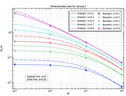
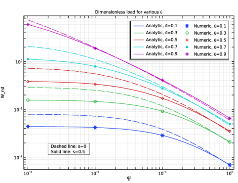
In the Settings window for 1D Plot Group, type Dimensionless Load vs. Psi: s=0.25 in the Label text field.
3
Locate the Data section. From the Dataset list, choose None.
4
Locate the Title section. From the Title type list, choose Manual.
5
In the Title text area, type Dimensionless load for various \epsilon.
6
Locate the Plot Settings section.
7
Select the x-axis label checkbox. In the associated text field, type \Psi.
8
Select the y-axis label checkbox. In the associated text field, type W_nd.
9
Locate the Axis section. Select the x-axis log scale checkbox.
10
Select the y-axis log scale checkbox.
11
Locate the Legend section. In the Number of columns text field, type 2.
12
In the Maximum relative width text field, type 1.
Function 1
1
In the Dimensionless Load vs. Psi: s=0.25 toolbar, click  More Plots and choose Function.
2
In the Settings window for Function, locate the Data section.
3
From the Dataset list, choose Grid 1D 2.
4
Locate the y-Axis Data section. In the Expression text field, type sqrt((integrate(integrate((24/pi^3)*sum(pbar_summand(0.1,n,Psi,0.25,theta,z),n,1,n_upper_lim)*cos(theta),theta,0,pi),z,-L/2,L/2))^2+(integrate(integrate((24/pi^3)*sum(pbar_summand(0.1,n,Psi,0.25,theta,z),n,1,n_upper_lim)*sin(theta),theta,0,pi),z,-L/2,L/2))^2)/L.
5
Locate the x-Axis Data section. In the Expression text field, type Psi.
6
In the Lower bound text field, type 0.001.
7
Locate the Coloring and Style section. From the Color list, choose Cycle (reset).
8
Locate the Legends section. Select the Show legends checkbox.
9
From the Legends list, choose Manual.
10
Function 2
1
Right-click Function 1 and choose Duplicate.
2
In the Settings window for Function, locate the y-Axis Data section.
3
In the Expression text field, type sqrt((integrate(integrate((24/pi^3)*sum(pbar_summand(0.3,n,Psi,0.25,theta,z),n,1,n_upper_lim)*cos(theta),theta,0,pi),z,-L/2,L/2))^2+(integrate(integrate((24/pi^3)*sum(pbar_summand(0.3,n,Psi,0.25,theta,z),n,1,n_upper_lim)*sin(theta),theta,0,pi),z,-L/2,L/2))^2)/L.
4
Locate the Coloring and Style section. From the Color list, choose Cycle.
5
Locate the Legends section. In the table, enter the following settings:
Function 3
1
Right-click Function 2 and choose Duplicate.
2
In the Settings window for Function, locate the y-Axis Data section.
3
In the Expression text field, type sqrt((integrate(integrate((24/pi^3)*sum(pbar_summand(0.5,n,Psi,0.25,theta,z),n,1,n_upper_lim)*cos(theta),theta,0,pi),z,-L/2,L/2))^2+(integrate(integrate((24/pi^3)*sum(pbar_summand(0.5,n,Psi,0.25,theta,z),n,1,n_upper_lim)*sin(theta),theta,0,pi),z,-L/2,L/2))^2)/L.
4
Locate the Legends section. In the table, enter the following settings:
Function 4
1
Right-click Function 3 and choose Duplicate.
2
In the Settings window for Function, locate the y-Axis Data section.
3
In the Expression text field, type sqrt((integrate(integrate((24/pi^3)*sum(pbar_summand(0.7,n,Psi,0.25,theta,z),n,1,n_upper_lim)*cos(theta),theta,0,pi),z,-L/2,L/2))^2+(integrate(integrate((24/pi^3)*sum(pbar_summand(0.7,n,Psi,0.25,theta,z),n,1,n_upper_lim)*sin(theta),theta,0,pi),z,-L/2,L/2))^2)/L.
4
Locate the Legends section. In the table, enter the following settings:
Function 5
1
Right-click Function 4 and choose Duplicate.
2
In the Settings window for Function, locate the y-Axis Data section.
3
In the Expression text field, type sqrt((integrate(integrate((24/pi^3)*sum(pbar_summand(0.9,n,Psi,0.25,theta,z),n,1,n_upper_lim)*cos(theta),theta,0,pi),z,-L/2,L/2))^2+(integrate(integrate((24/pi^3)*sum(pbar_summand(0.9,n,Psi,0.25,theta,z),n,1,n_upper_lim)*sin(theta),theta,0,pi),z,-L/2,L/2))^2)/L.
4
Locate the Legends section. In the table, enter the following settings:
Dimensionless Load vs. Psi: s=0.25
In the Model Builder window, click Dimensionless Load vs. Psi: s=0.25.
Function 6
1
In the Dimensionless Load vs. Psi: s=0.25 toolbar, click  More Plots and choose Function.
2
In the Settings window for Function, locate the Data section.
3
From the Dataset list, choose Grid 1D 2.
4
Locate the y-Axis Data section. In the Expression text field, type sqrt((integrate(integrate((24/pi^3)*sum(pbar_summand(0.1,n,Psi,0,theta,z),n,1,n_upper_lim)*cos(theta),theta,0,pi),z,-L/2,L/2))^2+(integrate(integrate((24/pi^3)*sum(pbar_summand(0.1,n,Psi,0,theta,z),n,1,n_upper_lim)*sin(theta),theta,0,pi),z,-L/2,L/2))^2)/L.
5
Locate the x-Axis Data section. In the Expression text field, type Psi.
6
In the Lower bound text field, type 0.001.
7
Locate the Coloring and Style section. Find the Line style subsection. From the Line list, choose Dashed.
8
From the Color list, choose Cycle (reset).
Function 7
1
Right-click Function 6 and choose Duplicate.
2
In the Settings window for Function, locate the y-Axis Data section.
3
In the Expression text field, type sqrt((integrate(integrate((24/pi^3)*sum(pbar_summand(0.3,n,Psi,0,theta,z),n,1,n_upper_lim)*cos(theta),theta,0,pi),z,-L/2,L/2))^2+(integrate(integrate((24/pi^3)*sum(pbar_summand(0.3,n,Psi,0,theta,z),n,1,n_upper_lim)*sin(theta),theta,0,pi),z,-L/2,L/2))^2)/L.
4
Locate the Coloring and Style section. From the Color list, choose Cycle.
Function 8
1
Right-click Function 7 and choose Duplicate.
2
In the Settings window for Function, locate the y-Axis Data section.
3
In the Expression text field, type sqrt((integrate(integrate((24/pi^3)*sum(pbar_summand(0.5,n,Psi,0,theta,z),n,1,n_upper_lim)*cos(theta),theta,0,pi),z,-L/2,L/2))^2+(integrate(integrate((24/pi^3)*sum(pbar_summand(0.5,n,Psi,0,theta,z),n,1,n_upper_lim)*sin(theta),theta,0,pi),z,-L/2,L/2))^2)/L.
Function 9
1
Right-click Function 8 and choose Duplicate.
2
In the Settings window for Function, locate the y-Axis Data section.
3
In the Expression text field, type sqrt((integrate(integrate((24/pi^3)*sum(pbar_summand(0.7,n,Psi,0,theta,z),n,1,n_upper_lim)*cos(theta),theta,0,pi),z,-L/2,L/2))^2+(integrate(integrate((24/pi^3)*sum(pbar_summand(0.7,n,Psi,0,theta,z),n,1,n_upper_lim)*sin(theta),theta,0,pi),z,-L/2,L/2))^2)/L.
Function 10
1
Right-click Function 9 and choose Duplicate.
2
In the Settings window for Function, locate the y-Axis Data section.
3
In the Expression text field, type sqrt((integrate(integrate((24/pi^3)*sum(pbar_summand(0.9,n,Psi,0,theta,z),n,1,n_upper_lim)*cos(theta),theta,0,pi),z,-L/2,L/2))^2+(integrate(integrate((24/pi^3)*sum(pbar_summand(0.9,n,Psi,0,theta,z),n,1,n_upper_lim)*sin(theta),theta,0,pi),z,-L/2,L/2))^2)/L.
Table Graph 1
1
In the Model Builder window, right-click Dimensionless Load vs. Psi: s=0.25 and choose Table Graph.
2
In the Settings window for Table Graph, locate the Data section.
3
From the Table list, choose Table 5.
4
From the x-axis data list, choose Psi.
5
From the Plot columns list, choose Manual.
6
In the Columns list box, select (C^2/(mu*U*L^3))*sqrt((intop1(pfilm*cos(theta)))^2+(intop1(pfilm*sin(theta)))^2) (1).
7
Locate the Coloring and Style section. Find the Line style subsection. From the Line list, choose None.
8
From the Color list, choose Cycle (reset).
9
Find the Line markers subsection. From the Marker list, choose Cycle (reset).
10
Locate the Legends section. Select the Show legends checkbox.
11
From the Legends list, choose Manual.
12
Table Graph 2
1
Right-click Table Graph 1 and choose Duplicate.
2
In the Settings window for Table Graph, locate the Data section.
3
From the Table list, choose Table 6.
4
Locate the Coloring and Style section. From the Color list, choose Cycle.
5
Find the Line markers subsection. From the Marker list, choose Cycle.
6
Locate the Legends section. In the table, enter the following settings:
Table Graph 3
1
Right-click Table Graph 2 and choose Duplicate.
2
In the Settings window for Table Graph, locate the Data section.
3
From the Table list, choose Table 7.
4
Locate the Legends section. In the table, enter the following settings:
Table Graph 4
1
Right-click Table Graph 3 and choose Duplicate.
2
In the Settings window for Table Graph, locate the Data section.
3
From the Table list, choose Table 8.
4
Locate the Legends section. In the table, enter the following settings:
Table Graph 5
1
Right-click Table Graph 4 and choose Duplicate.
2
In the Settings window for Table Graph, locate the Data section.
3
From the Table list, choose Table 9.
4
Locate the Legends section. In the table, enter the following settings:
Annotation 1
1
In the Model Builder window, right-click Dimensionless Load vs. Psi: s=0.25 and choose Annotation.
2
In the Settings window for Annotation, locate the Data section.
3
From the Dataset list, choose Study 1/Solution 1 (sol1).
4
Locate the Annotation section. In the Text text field, type Dashed line: s=0\\Solid line: s=0.25.
5
Select the LaTeX markup checkbox.
6
Locate the Position section. In the X text field, type 0.002.
7
In the Y text field, type 0.02.
8
Locate the Coloring and Style section. Clear the Show point checkbox.
9
Select the Show frame checkbox.
Dimensionless Load vs. Psi: s=0.25
1
In the Model Builder window, click Dimensionless Load vs. Psi: s=0.25.
2
In the Dimensionless Load vs. Psi: s=0.25 toolbar, click  Plot.
Dimensionless Load vs. ep: s=0.5
1
In the Results toolbar, click  1D Plot Group.
2
In the Settings window for 1D Plot Group, type Dimensionless Load vs. ep: s=0.5 in the Label text field.
3
Locate the Data section. From the Dataset list, choose None.
4
Locate the Title section. From the Title type list, choose Manual.
5
In the Title text area, type Dimensionless load for various \Psi.
6
Locate the Plot Settings section.
7
Select the x-axis label checkbox. In the associated text field, type \epsilon.
8
Select the y-axis label checkbox. In the associated text field, type W_nd.
9
Locate the Axis section. Select the y-axis log scale checkbox.
10
Locate the Legend section. From the Position list, choose Lower right.
11
In the Number of columns text field, type 2.
12
In the Maximum relative width text field, type 1.
Function 1
1
In the Dimensionless Load vs. ep: s=0.5 toolbar, click  More Plots and choose Function.
2
In the Settings window for Function, locate the Data section.
3
From the Dataset list, choose Grid 1D 1.
4
Locate the y-Axis Data section. In the Expression text field, type (C^2/(mu*U*L^3))*sqrt((integrate(integrate(((mu*U*L^2)/(R*C^2))*(24/pi^3)*sum((-1)^(n+1)*ep*g_n(ep,n,1,0.5,theta)*cos(pi*beta_n(n)*z/L)/(2*n-1)^3,n,1,n_upper_lim)*cos(theta)*R,theta,0,pi),z,-L/2,L/2))^2+(integrate(integrate(((mu*U*L^2)/(R*C^2))*(24/pi^3)*sum((-1)^(n+1)*ep*g_n(ep,n,1,0.5,theta)*cos(pi*beta_n(n)*z/L)/(2*n-1)^3,n,1,n_upper_lim)*sin(theta)*R,theta,0,pi),z,-L/2,L/2))^2).
5
Locate the x-Axis Data section. In the Expression text field, type ep.
6
Locate the Coloring and Style section. From the Color list, choose Cycle (reset).
7
Locate the Legends section. Select the Show legends checkbox.
8
From the Legends list, choose Manual.
9
Function 2
1
Right-click Function 1 and choose Duplicate.
2
In the Settings window for Function, locate the y-Axis Data section.
3
In the Expression text field, type (C^2/(mu*U*L^3))*sqrt((integrate(integrate(((mu*U*L^2)/(R*C^2))*(24/pi^3)*sum((-1)^(n+1)*ep*g_n(ep,n,0.1,0.5,theta)*cos(pi*beta_n(n)*z/L)/(2*n-1)^3,n,1,n_upper_lim)*cos(theta)*R,theta,0,pi),z,-L/2,L/2))^2+(integrate(integrate(((mu*U*L^2)/(R*C^2))*(24/pi^3)*sum((-1)^(n+1)*ep*g_n(ep,n,0.1,0.5,theta)*cos(pi*beta_n(n)*z/L)/(2*n-1)^3,n,1,n_upper_lim)*sin(theta)*R,theta,0,pi),z,-L/2,L/2))^2).
4
Locate the Coloring and Style section. From the Color list, choose Cycle.
5
Locate the Legends section. In the table, enter the following settings:
Function 3
1
Right-click Function 2 and choose Duplicate.
2
In the Settings window for Function, locate the y-Axis Data section.
3
In the Expression text field, type (C^2/(mu*U*L^3))*sqrt((integrate(integrate(((mu*U*L^2)/(R*C^2))*(24/pi^3)*sum((-1)^(n+1)*ep*g_n(ep,n,0.01,0.5,theta)*cos(pi*beta_n(n)*z/L)/(2*n-1)^3,n,1,n_upper_lim)*cos(theta)*R,theta,0,pi),z,-L/2,L/2))^2+(integrate(integrate(((mu*U*L^2)/(R*C^2))*(24/pi^3)*sum((-1)^(n+1)*ep*g_n(ep,n,0.01,0.5,theta)*cos(pi*beta_n(n)*z/L)/(2*n-1)^3,n,1,n_upper_lim)*sin(theta)*R,theta,0,pi),z,-L/2,L/2))^2).
4
Locate the Legends section. In the table, enter the following settings:
Function 4
1
Right-click Function 3 and choose Duplicate.
2
In the Settings window for Function, locate the y-Axis Data section.
3
In the Expression text field, type (C^2/(mu*U*L^3))*sqrt((integrate(integrate(((mu*U*L^2)/(R*C^2))*(24/pi^3)*sum((-1)^(n+1)*ep*g_n(ep,n,0.001,0.5,theta)*cos(pi*beta_n(n)*z/L)/(2*n-1)^3,n,1,n_upper_lim)*cos(theta)*R,theta,0,pi),z,-L/2,L/2))^2+(integrate(integrate(((mu*U*L^2)/(R*C^2))*(24/pi^3)*sum((-1)^(n+1)*ep*g_n(ep,n,0.001,0.5,theta)*cos(pi*beta_n(n)*z/L)/(2*n-1)^3,n,1,n_upper_lim)*sin(theta)*R,theta,0,pi),z,-L/2,L/2))^2).
4
Locate the Legends section. In the table, enter the following settings:
Annotation 1, Function 5, Function 6, Function 7, Function 8, Table Graph 1, Table Graph 2, Table Graph 3, Table Graph 4
1
In the Model Builder window, under Results > Dimensionless Load vs. ep: s=0.25, Ctrl-click to select Function 5, Function 6, Function 7, Function 8, Table Graph 1, Table Graph 2, Table Graph 3, Table Graph 4, and Annotation 1.
2
Dimensionless Load vs. ep: s=0.5
In the Model Builder window, under Results right-click Dimensionless Load vs. ep: s=0.5 and choose Paste Multiple Items.
Table Graph 1
1
In the Settings window for Table Graph, locate the Data section.
2
From the Table list, choose Table 10.
Table Graph 2
1
In the Model Builder window, click Table Graph 2.
2
In the Settings window for Table Graph, locate the Data section.
3
From the Table list, choose Table 11.
Table Graph 3
1
In the Model Builder window, click Table Graph 3.
2
In the Settings window for Table Graph, locate the Data section.
3
From the Table list, choose Table 12.
Table Graph 4
1
In the Model Builder window, click Table Graph 4.
2
In the Settings window for Table Graph, locate the Data section.
3
From the Table list, choose Table 13.
Annotation 1
1
In the Model Builder window, click Annotation 1.
2
In the Settings window for Annotation, locate the Annotation section.
3
In the Text text field, type Dashed line: s=0\\Solid line: s=0.5.
Dimensionless Load vs. ep: s=0.5
1
In the Model Builder window, click Dimensionless Load vs. ep: s=0.5.
2
In the Dimensionless Load vs. ep: s=0.5 toolbar, click  Plot.
Dimensionless Load vs. Psi: s=0.5
1
In the Results toolbar, click  1D Plot Group.
2
In the Settings window for 1D Plot Group, type Dimensionless Load vs. Psi: s=0.5 in the Label text field.
3
Locate the Data section. From the Dataset list, choose None.
4
Locate the Title section. From the Title type list, choose Manual.
5
In the Title text area, type Dimensionless load for various \epsilon.
6
Locate the Plot Settings section.
7
Select the x-axis label checkbox. In the associated text field, type \Psi.
8
Select the y-axis label checkbox. In the associated text field, type W_nd.
9
Locate the Axis section. Select the y-axis log scale checkbox.
10
Select the x-axis log scale checkbox.
11
Locate the Legend section. In the Number of columns text field, type 2.
12
In the Maximum relative width text field, type 1.
Function 1
1
In the Dimensionless Load vs. Psi: s=0.5 toolbar, click  More Plots and choose Function.
2
In the Settings window for Function, locate the Data section.
3
From the Dataset list, choose Grid 1D 2.
4
Locate the y-Axis Data section. In the Expression text field, type (C^2/(mu*U*L^3))*sqrt((integrate(integrate(((mu*U*L^2)/(R*C^2))*(24/pi^3)*sum((-1)^(n+1)*0.1*g_n(0.1,n,Psi,0.5,theta)*cos(pi*beta_n(n)*z/L)/(2*n-1)^3,n,1,n_upper_lim)*cos(theta)*R,theta,0,pi),z,-L/2,L/2))^2+(integrate(integrate(((mu*U*L^2)/(R*C^2))*(24/pi^3)*sum((-1)^(n+1)*0.1*g_n(0.1,n,Psi,0.5,theta)*cos(pi*beta_n(n)*z/L)/(2*n-1)^3,n,1,n_upper_lim)*sin(theta)*R,theta,0,pi),z,-L/2,L/2))^2).
5
Locate the x-Axis Data section. In the Expression text field, type Psi.
6
In the Lower bound text field, type 0.001.
7
Locate the Coloring and Style section. From the Color list, choose Cycle (reset).
8
Locate the Legends section. Select the Show legends checkbox.
9
From the Legends list, choose Manual.
10
Function 2
1
Right-click Function 1 and choose Duplicate.
2
In the Settings window for Function, locate the y-Axis Data section.
3
In the Expression text field, type (C^2/(mu*U*L^3))*sqrt((integrate(integrate(((mu*U*L^2)/(R*C^2))*(24/pi^3)*sum((-1)^(n+1)*0.3*g_n(0.3,n,Psi,0.5,theta)*cos(pi*beta_n(n)*z/L)/(2*n-1)^3,n,1,n_upper_lim)*cos(theta)*R,theta,0,pi),z,-L/2,L/2))^2+(integrate(integrate(((mu*U*L^2)/(R*C^2))*(24/pi^3)*sum((-1)^(n+1)*0.3*g_n(0.3,n,Psi,0.5,theta)*cos(pi*beta_n(n)*z/L)/(2*n-1)^3,n,1,n_upper_lim)*sin(theta)*R,theta,0,pi),z,-L/2,L/2))^2).
4
Locate the Coloring and Style section. From the Color list, choose Cycle.
5
Locate the Legends section. In the table, enter the following settings:
Function 3
1
Right-click Function 2 and choose Duplicate.
2
In the Settings window for Function, locate the y-Axis Data section.
3
In the Expression text field, type (C^2/(mu*U*L^3))*sqrt((integrate(integrate(((mu*U*L^2)/(R*C^2))*(24/pi^3)*sum((-1)^(n+1)*0.5*g_n(0.5,n,Psi,0.5,theta)*cos(pi*beta_n(n)*z/L)/(2*n-1)^3,n,1,n_upper_lim)*cos(theta)*R,theta,0,pi),z,-L/2,L/2))^2+(integrate(integrate(((mu*U*L^2)/(R*C^2))*(24/pi^3)*sum((-1)^(n+1)*0.5*g_n(0.5,n,Psi,0.5,theta)*cos(pi*beta_n(n)*z/L)/(2*n-1)^3,n,1,n_upper_lim)*sin(theta)*R,theta,0,pi),z,-L/2,L/2))^2).
4
Locate the Legends section. In the table, enter the following settings:
Function 4
1
Right-click Function 3 and choose Duplicate.
2
In the Settings window for Function, locate the y-Axis Data section.
3
In the Expression text field, type (C^2/(mu*U*L^3))*sqrt((integrate(integrate(((mu*U*L^2)/(R*C^2))*(24/pi^3)*sum((-1)^(n+1)*0.7*g_n(0.7,n,Psi,0.5,theta)*cos(pi*beta_n(n)*z/L)/(2*n-1)^3,n,1,n_upper_lim)*cos(theta)*R,theta,0,pi),z,-L/2,L/2))^2+(integrate(integrate(((mu*U*L^2)/(R*C^2))*(24/pi^3)*sum((-1)^(n+1)*0.7*g_n(0.7,n,Psi,0.5,theta)*cos(pi*beta_n(n)*z/L)/(2*n-1)^3,n,1,n_upper_lim)*sin(theta)*R,theta,0,pi),z,-L/2,L/2))^2).
4
Locate the Legends section. In the table, enter the following settings:
Function 5
1
Right-click Function 4 and choose Duplicate.
2
In the Settings window for Function, locate the y-Axis Data section.
3
In the Expression text field, type (C^2/(mu*U*L^3))*sqrt((integrate(integrate(((mu*U*L^2)/(R*C^2))*(24/pi^3)*sum((-1)^(n+1)*0.9*g_n(0.9,n,Psi,0.5,theta)*cos(pi*beta_n(n)*z/L)/(2*n-1)^3,n,1,n_upper_lim)*cos(theta)*R,theta,0,pi),z,-L/2,L/2))^2+(integrate(integrate(((mu*U*L^2)/(R*C^2))*(24/pi^3)*sum((-1)^(n+1)*0.9*g_n(0.9,n,Psi,0.5,theta)*cos(pi*beta_n(n)*z/L)/(2*n-1)^3,n,1,n_upper_lim)*sin(theta)*R,theta,0,pi),z,-L/2,L/2))^2).
4
Locate the Legends section. In the table, enter the following settings:
Annotation 1, Function 10, Function 6, Function 7, Function 8, Function 9, Table Graph 1, Table Graph 2, Table Graph 3, Table Graph 4, Table Graph 5
1
In the Model Builder window, under Results > Dimensionless Load vs. Psi: s=0.25, Ctrl-click to select Function 6, Function 7, Function 8, Function 9, Function 10, Table Graph 1, Table Graph 2, Table Graph 3, Table Graph 4, Table Graph 5, and Annotation 1.
2
Dimensionless Load vs. Psi: s=0.5
In the Model Builder window, under Results right-click Dimensionless Load vs. Psi: s=0.5 and choose Paste Multiple Items.
Table Graph 1
1
In the Settings window for Table Graph, locate the Data section.
2
From the Table list, choose Table 14.
Table Graph 2
1
In the Model Builder window, click Table Graph 2.
2
In the Settings window for Table Graph, locate the Data section.
3
From the Table list, choose Table 15.
Table Graph 3
1
In the Model Builder window, click Table Graph 3.
2
In the Settings window for Table Graph, locate the Data section.
3
From the Table list, choose Table 16.
Table Graph 4
1
In the Model Builder window, click Table Graph 4.
2
In the Settings window for Table Graph, locate the Data section.
3
From the Table list, choose Table 17.
Table Graph 5
1
In the Model Builder window, click Table Graph 5.
2
In the Settings window for Table Graph, locate the Data section.
3
From the Table list, choose Table 18.
Annotation 1
1
In the Model Builder window, click Annotation 1.
2
In the Settings window for Annotation, locate the Annotation section.
3
In the Text text field, type Dashed line: s=0\\Solid line: s=0.5.
Dimensionless Load vs. Psi: s=0.5
1
In the Model Builder window, click Dimensionless Load vs. Psi: s=0.5.
2
In the Dimensionless Load vs. Psi: s=0.5 toolbar, click  Plot.
Attitude Angle vs. ep: s=0.25
1
In the Results toolbar, click  Polar Plot Group.
2
In the Settings window for Polar Plot Group, type Attitude Angle vs. Psi in the Label text field.
3
Locate the Data section. From the Dataset list, choose None.
4
Click to expand the Title section. From the Title type list, choose Manual.
5
In the Title text area, type Attitude angle for various \Psi.
6
Locate the Axis section. From the Zero angle list, choose Down.
7
From the Rotation direction list, choose Clockwise.
8
Locate the Legend section. In the Number of columns text field, type 2.
9
In the Maximum relative width text field, type 1.
10
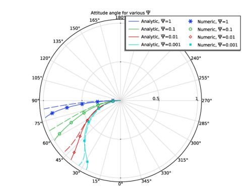
Click to expand the Window Settings section. In the Label text field, type Attitude Angle vs. ep: s=0.25.
Line Graph 1
1
Right-click Attitude Angle vs. ep: s=0.25 and choose Line Graph.
2
In the Settings window for Line Graph, locate the Data section.
3
From the Dataset list, choose Grid 1D 1.
4
Locate the r-Axis Data section. In the Expression text field, type ep.
5
Locate the θ Angle Data section. From the Parameter list, choose Expression.
6
In the Expression text field, type atan(-(integrate(integrate((24/pi^3)*sum(pbar_summand(ep,n,1,0.25,theta,z),n,1,n_upper_lim)*sin(theta),theta,0,pi),z,-L/2,L/2))/(integrate(integrate((24/pi^3)*sum(pbar_summand(ep,n,1,0.25,theta,z),n,1,n_upper_lim)*cos(theta),theta,0,pi),z,-L/2,L/2))).
7
Click to expand the Coloring and Style section. From the Color list, choose Cycle (reset).
8
Click to expand the Legends section. Select the Show legends checkbox.
9
From the Legends list, choose Manual.
10
Line Graph 2
1
Right-click Line Graph 1 and choose Duplicate.
2
In the Settings window for Line Graph, locate the θ Angle Data section.
3
In the Expression text field, type atan(-(integrate(integrate((24/pi^3)*sum(pbar_summand(ep,n,0.1,0.25,theta,z),n,1,n_upper_lim)*sin(theta),theta,0,pi),z,-L/2,L/2))/(integrate(integrate((24/pi^3)*sum(pbar_summand(ep,n,0.1,0.25,theta,z),n,1,n_upper_lim)*cos(theta),theta,0,pi),z,-L/2,L/2))).
4
Locate the Coloring and Style section. From the Color list, choose Cycle.
5
Locate the Legends section. In the table, enter the following settings:
Line Graph 3
1
Right-click Line Graph 2 and choose Duplicate.
2
In the Settings window for Line Graph, locate the θ Angle Data section.
3
In the Expression text field, type atan(-(integrate(integrate((24/pi^3)*sum(pbar_summand(ep,n,0.01,0.25,theta,z),n,1,n_upper_lim)*sin(theta),theta,0,pi),z,-L/2,L/2))/(integrate(integrate((24/pi^3)*sum(pbar_summand(ep,n,0.01,0.25,theta,z),n,1,n_upper_lim)*cos(theta),theta,0,pi),z,-L/2,L/2))).
4
Locate the Legends section. In the table, enter the following settings:
Line Graph 4
1
Right-click Line Graph 3 and choose Duplicate.
2
In the Settings window for Line Graph, locate the θ Angle Data section.
3
In the Expression text field, type atan(-(integrate(integrate((24/pi^3)*sum(pbar_summand(ep,n,0.001,0.25,theta,z),n,1,n_upper_lim)*sin(theta),theta,0,pi),z,-L/2,L/2))/(integrate(integrate((24/pi^3)*sum(pbar_summand(ep,n,0.001,0.25,theta,z),n,1,n_upper_lim)*cos(theta),theta,0,pi),z,-L/2,L/2))).
4
Locate the Legends section. In the table, enter the following settings:
Line Graph 5
1
In the Model Builder window, right-click Attitude Angle vs. ep: s=0.25 and choose Line Graph.
2
In the Settings window for Line Graph, locate the Data section.
3
From the Dataset list, choose Grid 1D 1.
4
Locate the r-Axis Data section. In the Expression text field, type ep.
5
Locate the θ Angle Data section. From the Parameter list, choose Expression.
6
In the Expression text field, type atan(-(integrate(integrate((24/pi^3)*sum(pbar_summand(ep,n,1,0,theta,z),n,1,n_upper_lim)*sin(theta),theta,0,pi),z,-L/2,L/2))/(integrate(integrate((24/pi^3)*sum(pbar_summand(ep,n,1,0,theta,z),n,1,n_upper_lim)*cos(theta),theta,0,pi),z,-L/2,L/2))).
7
Locate the Coloring and Style section. Find the Line style subsection. From the Line list, choose Dashed.
8
From the Color list, choose Cycle (reset).
Line Graph 6
1
Right-click Line Graph 5 and choose Duplicate.
2
In the Settings window for Line Graph, locate the Coloring and Style section.
3
From the Color list, choose Cycle.
4
Locate the θ Angle Data section. In the Expression text field, type atan(-(integrate(integrate((24/pi^3)*sum(pbar_summand(ep,n,0.1,0,theta,z),n,1,n_upper_lim)*sin(theta),theta,0,pi),z,-L/2,L/2))/(integrate(integrate((24/pi^3)*sum(pbar_summand(ep,n,0.1,0,theta,z),n,1,n_upper_lim)*cos(theta),theta,0,pi),z,-L/2,L/2))).
Line Graph 7
1
Right-click Line Graph 6 and choose Duplicate.
2
In the Settings window for Line Graph, locate the θ Angle Data section.
3
In the Expression text field, type atan(-(integrate(integrate((24/pi^3)*sum(pbar_summand(ep,n,0.01,0,theta,z),n,1,n_upper_lim)*sin(theta),theta,0,pi),z,-L/2,L/2))/(integrate(integrate((24/pi^3)*sum(pbar_summand(ep,n,0.01,0,theta,z),n,1,n_upper_lim)*cos(theta),theta,0,pi),z,-L/2,L/2))).
Line Graph 8
1
Right-click Line Graph 7 and choose Duplicate.
2
In the Settings window for Line Graph, locate the θ Angle Data section.
3
In the Expression text field, type atan(-(integrate(integrate((24/pi^3)*sum(pbar_summand(ep,n,0.001,0,theta,z),n,1,n_upper_lim)*sin(theta),theta,0,pi),z,-L/2,L/2))/(integrate(integrate((24/pi^3)*sum(pbar_summand(ep,n,0.001,0,theta,z),n,1,n_upper_lim)*cos(theta),theta,0,pi),z,-L/2,L/2))).
Table Graph 1
1
In the Model Builder window, right-click Attitude Angle vs. ep: s=0.25 and choose Table Graph.
2
In the Settings window for Table Graph, locate the Data section.
3
From the θ angle data list, choose atan(-(intop1(pfilm*sin(theta)))/(intop1(pfilm*cos(theta)))) (rad).
4
From the Plot columns list, choose Manual.
5
In the Columns list box, select ep.
6
Locate the Coloring and Style section. Find the Line style subsection. From the Line list, choose None.
7
From the Color list, choose Cycle (reset).
8
Find the Line markers subsection. From the Marker list, choose Cycle (reset).
9
Click to expand the Legends section. Select the Show legends checkbox.
10
From the Legends list, choose Manual.
11
Table Graph 2
1
Right-click Table Graph 1 and choose Duplicate.
2
In the Settings window for Table Graph, locate the Data section.
3
From the Table list, choose Table 2.
4
Locate the Coloring and Style section. From the Color list, choose Cycle.
5
Find the Line markers subsection. From the Marker list, choose Cycle.
6
Locate the Legends section. In the table, enter the following settings:
Table Graph 3
1
Right-click Table Graph 2 and choose Duplicate.
2
In the Settings window for Table Graph, locate the Data section.
3
From the Table list, choose Table 3.
4
Locate the Legends section. In the table, enter the following settings:
Table Graph 4
1
Right-click Table Graph 3 and choose Duplicate.
2
In the Settings window for Table Graph, locate the Data section.
3
From the Table list, choose Table 4.
4
Locate the Legends section. In the table, enter the following settings:
Attitude Angle vs. ep: s=0.25
1
In the Model Builder window, click Attitude Angle vs. ep: s=0.25.
2
In the Attitude Angle vs. ep: s=0.25 toolbar, click  Plot.
Darcy’s Velocity Streamlines, Film Pressure Contour and Film Thickness
1
In the Results toolbar, click  3D Plot Group.
2
In the Settings window for 3D Plot Group, locate the Data section.
3
From the Dataset list, choose Study 2/Solution 43 (sol43).
4
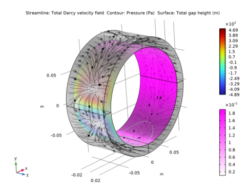
In the Label text field, type Darcy's Velocity Streamlines, Film Pressure Contour and Film Thickness.
5
Locate the Color Legend section. From the Position list, choose Right double.
Streamline 1
1
Right-click Darcy’s Velocity Streamlines, Film Pressure Contour and Film Thickness and choose Streamline.
2
In the Settings window for Streamline, locate the Expression section.
3
In the X-component text field, type dl.u.
4
In the Y-component text field, type dl.v.
5
In the Z-component text field, type dl.w.
6
Click to expand the Title section. Locate the Streamline Positioning section. From the Positioning list, choose Uniform density.
7
Locate the Coloring and Style section. Find the Point style subsection. From the Type list, choose Arrow.
8
From the Color list, choose Black.
9
Locate the Streamline Positioning section. In the Density level text field, type 10.
Contour 1
1
In the Model Builder window, right-click Darcy’s Velocity Streamlines, Film Pressure Contour and Film Thickness and choose Contour.
2
In the Settings window for Contour, click to expand the Title section.
3
Locate the Levels section. In the Total levels text field, type 50.
4
Locate the Coloring and Style section. From the Legend type list, choose Filled.
Selection 1
1
Right-click Contour 1 and choose Selection.
2
In the Settings window for Selection, locate the Selection section.
3
Click  Paste Selection.
4
In the Paste Selection dialog, type 8, 9, 14, 16 in the Selection text field.
5
Surface 1
1
In the Model Builder window, right-click Darcy’s Velocity Streamlines, Film Pressure Contour and Film Thickness and choose Surface.
2
In the Settings window for Surface, locate the Expression section.
3
In the Expression text field, type tff.h.
4
Click to expand the Title section. Locate the Coloring and Style section. From the Coloring list, choose Gradient.
5
From the Top color list, choose Magenta.
6
From the Bottom color list, choose White.
7
From the Color table transformation list, choose None.
Selection 1
1
Right-click Surface 1 and choose Selection.
2
In the Settings window for Selection, locate the Selection section.
3
Click  Paste Selection.
4
In the Paste Selection dialog, type 8, 9, 14, 16 in the Selection text field.
5
Transparency 1
1
In the Model Builder window, right-click Surface 1 and choose Transparency.
2
In the Settings window for Transparency, locate the Transparency section.
3
Find the Transparency subsection. In the Transparency text field, type 0.1.
Surface 2
1
In the Model Builder window, right-click Darcy’s Velocity Streamlines, Film Pressure Contour and Film Thickness and choose Surface.
2
In the Settings window for Surface, locate the Expression section.
3
In the Expression text field, type 1.
4
Locate the Title section. From the Title type list, choose None.
5
Locate the Coloring and Style section. From the Coloring list, choose Uniform.
6
From the Color list, choose Gray.
Selection 1
1
Right-click Surface 2 and choose Selection.
2
In the Settings window for Selection, locate the Selection section.
3
Click  Paste Selection.
4
In the Paste Selection dialog, type 2-7, 11-13, 17-19 in the Selection text field.
5
Transparency 1
In the Model Builder window, right-click Surface 2 and choose Transparency.
Darcy’s Velocity Streamlines, Film Pressure Contour and Film Thickness
1
In the Settings window for 3D Plot Group, locate the Plot Settings section.
2
From the View list, choose New view.
3
In the Darcy’s Velocity Streamlines, Film Pressure Contour and Film Thickness toolbar, click  Plot.
Adjust the view to obtain Figure 8.