|
|
|
|
1
|
|
2
|
In the Select Physics tree, select Fluid Flow > Multiphase Flow > Phase Transport Mixture Model > Turbulent Flow > Turbulent Flow, k-ε.
|
|
3
|
Click Add.
|
|
4
|
Click
|
|
5
|
|
6
|
Click
|
|
1
|
|
2
|
Browse to the model’s Application Libraries folder and double-click the file sedimentation_ptmm_geom_sequence.mph.
|
|
3
|
|
1
|
|
2
|
On the object fin, select Boundaries 8, 10, and 11 only.
|
|
3
|
|
4
|
|
1
|
|
2
|
|
1
|
|
2
|
|
3
|
|
4
|
|
5
|
|
1
|
|
2
|
|
1
|
|
2
|
|
3
|
Select the Include gravity checkbox.
|
|
1
|
In the Model Builder window, under Component 1 (comp1) > Turbulent Flow, k-ε (spf) click Initial Values 1.
|
|
2
|
|
3
|
|
4
|
Clear the Compensate for hydrostatic pressure approximation checkbox.
|
|
1
|
|
2
|
|
3
|
|
1
|
|
3
|
|
4
|
|
5
|
|
6
|
|
7
|
In the text field, type 0.2*0.07.
|
|
8
|
|
9
|
|
10
|
|
11
|
Click OK.
|
|
12
|
|
13
|
|
1
|
|
3
|
|
4
|
From the list, choose Velocity.
|
|
5
|
|
6
|
Click to expand the Constraint Settings section. From the Apply reaction terms on list, choose All physics (symmetric).
|
|
1
|
|
3
|
|
4
|
|
1
|
|
3
|
|
4
|
Select the Phase s2 checkbox.
|
|
5
|
|
1
|
|
1
|
In the Model Builder window, under Component 1 (comp1) > Multiphysics click Mixture Model 1 (mfmm1).
|
|
3
|
|
4
|
|
5
|
Locate the Continuous Phase Properties section. From the ρc list, choose User defined. In the associated text field, type rho_c.
|
|
6
|
|
7
|
Locate the Dispersed Phase 2 Properties section. From the ρs2 list, choose User defined. In the associated text field, type rho_d.
|
|
8
|
|
1
|
|
2
|
|
3
|
From the list, choose User-controlled mesh.
|
|
1
|
|
2
|
|
3
|
|
1
|
|
2
|
|
3
|
|
1
|
|
2
|
|
3
|
|
4
|
|
6
|
|
7
|
|
1
|
|
2
|
|
3
|
|
4
|
|
5
|
|
1
|
|
2
|
|
3
|
|
4
|
|
5
|
|
1
|
In the Model Builder window, expand the Boundary Layers 1 node, then click Boundary Layer Properties 1.
|
|
2
|
|
3
|
|
4
|
|
5
|
Click
|
|
1
|
|
2
|
|
3
|
In the Output times text field, type range(0,0.01,0.1) range(1,10) 100*range(1,10) 1800*range(1,24).
|
|
1
|
|
2
|
|
3
|
In the Model Builder window, expand the Study 1 > Solver Configurations > Solution 1 (sol1) > Dependent Variables 1 node, then click Turbulent Dissipation Rate (comp1.ep).
|
|
4
|
|
5
|
|
6
|
|
7
|
In the Model Builder window, under Study 1 > Solver Configurations > Solution 1 (sol1) > Dependent Variables 1 click Turbulent Kinetic Energy (comp1.k).
|
|
8
|
|
9
|
|
10
|
|
11
|
In the Model Builder window, under Study 1 > Solver Configurations > Solution 1 (sol1) > Dependent Variables 1 click Pressure (comp1.p).
|
|
12
|
|
13
|
|
14
|
|
15
|
In the Model Builder window, under Study 1 > Solver Configurations > Solution 1 (sol1) > Dependent Variables 1 click Velocity Field (comp1.u).
|
|
16
|
|
17
|
|
18
|
In the Model Builder window, under Study 1 > Solver Configurations > Solution 1 (sol1) click Time-Dependent Solver 1.
|
|
19
|
|
20
|
|
21
|
In the Model Builder window, expand the Study 1 > Solver Configurations > Solution 1 (sol1) > Time-Dependent Solver 1 node, then click Segregated 1.
|
|
22
|
|
23
|
|
24
|
|
1
|
|
3
|
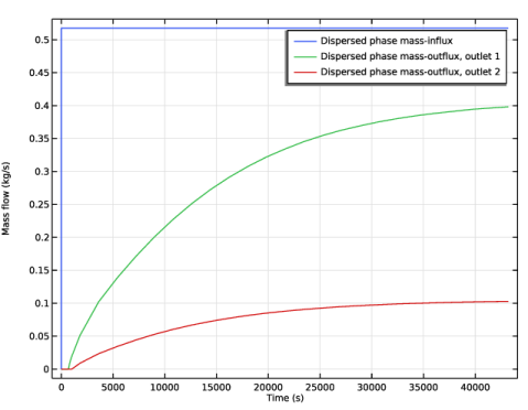
In the Settings window for Line Integration, click Replace Expression in the upper-right corner of the Expressions section. From the menu, choose Component 1 (comp1) > Phase Transport > Mass flux, phase s2 - kg/(m²·s) > phtr.Nz_s2 - Mass flux, phase s2, z-component.
|
|
4
|
Click
|
|
1
|
|
3
|
In the Settings window for Line Integration, click Replace Expression in the upper-right corner of the Expressions section. From the menu, choose Component 1 (comp1) > Phase Transport > Mass flux, phase s2 - kg/(m²·s) > phtr.Nz_s2 - Mass flux, phase s2, z-component.
|
|
4
|
Locate the Expressions section. In the table, enter the following settings:
|
|
5
|
|
1
|
|
2
|
|
3
|
In the Rename 1D Plot Group dialog, type Dispersed Phase In and Out Mass Fluxes in the New label text field.
|
|
4
|
Click OK.
|
|
5
|
|
6
|
|
7
|
|
1
|
|
2
|
|
3
|
Select the Show legends checkbox.
|
|
4
|
|
6
|
|
1
|
|
2
|
|
3
|
|
4
|
|
5
|
|
6
|
|
7
|
|
1
|
|
2
|
|
3
|
|
4
|
|
5
|
|
1
|
|
2
|
|
3
|
|
4
|
|
1
|
|
2
|
|
3
|
|
4
|
|
5
|
|
6
|
|
1
|
|
2
|
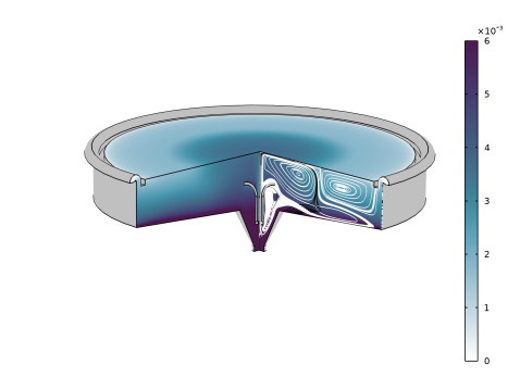
In the Settings window for Surface, click Replace Expression in the upper-right corner of the Expression section. From the menu, choose Component 1 (comp1) > Turbulent Flow, k-ε > Turbulence variables > spf.Delta_wPlus - Wall resolution in viscous units - 1.
|
|
3
|
|
4
|
|
1
|
|
2
|
In the Settings window for Streamline, click Replace Expression in the upper-right corner of the Expression section. From the menu, choose Component 1 (comp1) > Phase Transport > mfmm1.u_s2r,...,mfmm1.u_s2z - Convective velocity dispersed phase s2.
|
|
3
|
|
4
|
|
5
|
|
6
|
|
7
|
|
8
|
|
9
|
Locate the Coloring and Style section. Find the Point style subsection. From the Color list, choose Black.
|
|
1
|
|
2
|
In the Settings window for Streamline, click Replace Expression in the upper-right corner of the Expression section. From the menu, choose Component 1 (comp1) > Phase Transport > mfmm1.ucontr,...,mfmm1.ucontz - Velocity field, continuous phase.
|
|
3
|
|
4
|
|
5
|
|
6
|
|
7
|
|
8
|
|
9
|
Locate the Coloring and Style section. Find the Point style subsection. From the Color list, choose White.
|
|
1
|
|
2
|
|
3
|
|
4
|
|
5
|
|
6
|
|
7
|
|
8
|
|
1
|
|
2
|
|
4
|
Click
|
|
1
|
|
2
|
|
3
|
|
4
|
|
5
|
|
6
|
|
1
|
|
2
|
|
3
|
|
4
|
|
5
|
|
6
|
|
7
|
|
8
|
|
1
|
|
2
|
|
3
|
|
4
|
|
5
|
|
6
|
|
7
|
|
8
|
|
1
|
|
2
|
|
3
|
|
4
|
|
5
|
|
6
|
|
7
|
|
8
|
|
1
|
|
2
|
|
3
|
|
4
|
|
5
|
|
6
|
|
1
|
|
2
|
|
1
|
|
2
|
|
3
|
|
4
|
|
5
|
Click
|
|
1
|
|
2
|
|
3
|
|
4
|
|
5
|
|
6
|
|
7
|
Click
|
|
1
|
|
2
|
|
3
|
|
4
|
|
5
|
|
1
|
|
2
|
|
3
|
|
4
|
|
1
|
|
2
|
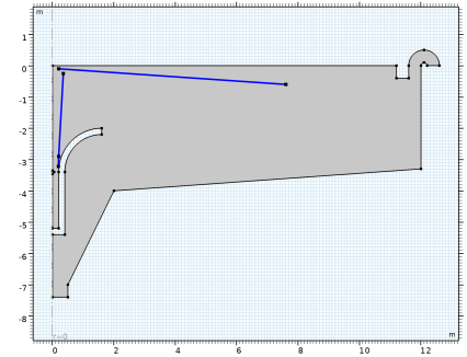
On the object r2, select Points 3 and 4 only.
|
|
3
|
|
4
|
|
1
|
|
2
|
|
3
|
|
4
|
|
1
|
|
2
|
|
3
|
|
4
|
|
5
|
Select the object c2 only.
|
|
6
|
Clear the Keep interior boundaries checkbox.
|
|
7
|
Click
|
|
1
|
|
2
|
|
4
|
Click
|
|
1
|
|
2
|
|
4
|
Click
|
|
1
|
|
2
|
|
4
|
Click
|
|
1
|
|
2
|