PDF

Spanwise Rotating Turbulent Channel Flow
Introduction
In this model, the Single-Phase Flow, Elliptic Blending R-ε interface is employed to investigate fully developed turbulent flow in a spanwise rotating planar channel, as well as the subsequent flow development in a suddenly expanded section. The dynamic characteristics of the resulting flows are analyzed in detail and visualized.
Model Definition
Correctly accounting for the impact of system rotation on turbulent flows is a challenge. Eddy-viscosity models are built so as to properly react to shear and strain but, commonly, not to vorticity. Activating Include rotation-curvature correction mends this deficiency to a certain extent. Nevertheless, the Reynolds stress tensor remains strictly proportional to the strain-rate tensor, which is too limiting in the general case. Differential Reynolds stress models of turbulence (RANS-RSM) are based on a deeper foundation, and appropriately respond both to the in-frame flow vorticity and to the frame rotation. However, even in the simplest case of a spanwise rotating turbulent channel, Wilcox R-ω and SSG-LRR underestimate the extent of the region with zero absolute vorticity, and predict laminarization at a too low rotation rate. Fortunately, the Elliptic Blending R-ε model from Ref. 1 properly blends turbulence behavior in the bulk and near-wall regions, which in turn leads to improved reaction to the system rotation.
In this example, spanwise rotating turbulent channel flow is extensively analyzed. The channel Reynolds number,
is Re = 14,000. Above, Ub is the streamwise bulk velocity and H is the height of the channel. The range of rotation numbers investigated,
is between Ro = 0 and Ro = 3 (note that Rossby number has the same denotation, Ro, although they are inverses of each other). Ω is the angular rotation rate. A Periodic Flow Condition in a geometry that is short in the streamwise direction is employed to compute the fully developed channel flow (periodic channel study). Then, the channel suddenly and symmetrically expands with a 1.5 height ratio. The deflection of the expanding jet and the asymmetry between the separation bubbles are the most apparent outcomes of the system rotation. The case Ro = 0.1 is presented below (expanded channel study).
Figure 1: The model geometry of the rotating periodic channel (top) and expanded rotating channel (bottom). The converged fully developed state of the periodic channel study is used as an inlet condition for the expanded channel study.
Assuming positive (counterclockwise, cyclonic) frame rotation and rightward flow direction, the Coriolis force acts downward. The in-frame flow vorticity is cyclonic near the top wall of the channel and anticyclonic near the bottom wall. At the anticyclonic side of the channel, turbulence is enhanced, while it is strongly suppressed at the cyclonic side. Correspondingly, the anticyclonic side is referred to as the “unstable side” and the cyclonic side as the “stable side”. In the central region of the turbulent channel flow (far away from the walls), the flow velocity possesses a constant cross-stream slope with the value of the anticyclonic in-frame vorticity, 2Ω, which exactly compensates the cyclonic vorticity, +2Ω, inherent to the system rotation.
Figure 2: Meshes used for the studies of the rotating periodic channel (top) and expanded channel (bottom). Very thin cells at the walls of the rotating channel are used to ensure accurate evaluation of traction. The initial developing region of the expanding jet is meshed fine, while the remaining near-outlet region serves mostly to reduce the effect of the outlet boundary condition.
Implementation in COMSOL Multiphysics
Figure 1 contains geometries along with boundary conditions for both studies, while Figure 2 presents the corresponding meshes. A Rotating Frame feature is employed to impose the frame rotation. It is crucial for the efficient computation of the periodic channel, since the Periodic Flow Condition feature is not inherently compatible with a moving wall-based approach. An Auxiliary sweep with continuation is used for quicker computation through the bunch of rotation numbers. The expanded channel flow is computed subsequently; values of variables at its inlet are taken from the converged state of the periodic channel flow. Thus, the inlet represents a fully developed turbulent channel flow in the rotating frame. The near-wall cells of the channel should be meshed very well, and the regions with separation bubbles and the ensuing wake should have very fine or at least fine meshing. The remaining part mainly serves to relieve the influence of the outlet boundary condition and might have quite coarse mesh. The pressure at the outlet is taken as if a Coriolis force of a constant velocity flow would be balanced by the cross-stream pressure gradient. Note that Use reduced pressure is activated to filter out centrifugal pressure.
The details of the implementation of the Single-Phase Flow, Elliptic Blending R-ε interface can be found in the section Theory for the Turbulent Flow Interfaces of the CFD Module User’s Guide, while specifics of the Rotating Frame feature are listed in Rotating Frame description of Theory for the Single-Phase Flow Interfaces.
Results and Discussion
Figure 3 shows velocity profiles in rotating turbulent channel flow. With increasing Ro, the profiles first become anticyclonically skewed with boosted slopes near the anticyclonic (unstable) wall and reduced slopes near the cyclonic (stable) wall. Consequently, the velocity maximum moves closer to the stable wall; for Ro in the interval (0.3, 1.1) the position of the maximum is at y > H/4, which means that it is near the stable side within one-quarter of H. At higher rotation rate, say at Ro larger than 1.1, the profiles show a clear tendency to laminarization, taking on progressively more parabolic form. At Ro = 3, laminarization is almost complete. Note that at small Ro the increase in the velocity slope near the unstable side is much less visible than the slope’s decrease near the stable wall.
Figure 3: Rotating channel flow at various rotation numbers Ro: velocity profiles. The channel is situated within [H/2,H/2].
Indeed, Figure 4 presents the dependence of the friction velocity uτ = τw on Ro (normalized by the nonrotating value). Clearly, while uτ at the unstable side grows only slightly with Ro (by 10% at Ro = 0.1), uτ at the stable side falls abruptly (by 42% at Ro = 0.2). The picture is consistent with Ref. 1. The stable-side plunge in uτ has correct magnitude, but happens too quickly (Ro = 0.5 is an approximate rotation number when uτ reduces by 42% according to Large-Eddy Simulation).
Figure 5 illustrates flow pattern in a suddenly expanded channel section at Ro = 0.1 (rotation number is based on the parameters of the periodic channel). The jet becomes quickly deflected to the unstable side by the Coriolis force, and then slowly approaches strictly straight direction in the expanded section. Apparently, two major separation bubbles are formed. The one at the unstable wall is quite compact, shorter than in nonrotating case, with easily distinguishable boundary. Meantime, that on the stable wall is very extended in the streamwise direction and has long fuzzy streaks, which make it hard to determine reconnection point visually. Indeed, according to Ref. 1, the Elliptic Blending R-ε model accurately reproduces behavior on the unstable side, but is less reliable at the stable side of the expanded channel setup. Allegedly, imperfect sensitivity of the model to the laminarization tendency is responsible for this. It might be suggested that true longitudinal length of the stable-side bubble is approximately half the length predicted by the current version of the Elliptic Blending R-ε. The major bubbles are accompanied by small counterrotating secondary “corner” bubbles (pushed to the corners of the expanded channel).
Figure 4: Rotating channel flow at various rotation numbers Ro: uτ(Ro)/uτ(0) is presented; y is within [H/2,H/2].
Figure 6 shows friction coefficients along the stable and unstable walls of the expanded section,
with streamwise length normalized by the step height hstep. Notice that even on unstable side it takes quite a distance before friction coefficient magnitude settles to a constant value. On the stable side Cf is negative for very long stretch, which indicates that the turbulence model overestimates rotation-induced tendency to laminarization. Thus, flow recovery to the new fully developed state is significantly delayed. The friction coefficient variations inside the secondary bubbles are also revealed.
Figure 5: Suddenly expanded rotating channel. The jet is deflected down by the Coriolis force, the negative maximum of the y-velocity is twice higher than its positive maximum, and two different separation regions are formed. The separation regions are in color, and each consists of a major bubble and a counterrotating secondary“corner bubble”. Re = 14,000 and Ro = 0.1(parameters for the periodic channel).
Figure 6: Friction coefficients along the walls of the expanded channel at Re = 14,000 and Ro = 0.1(parameters for the narrower section). The length is normalized by the step height hstep = (Hexp − H)/2.
Figure 7 illustrates contours of reduced pressure, which are almost perpendicular to the Coriolis force and are strongly distorted by the minima associated with pressure losses in the separation regions. The trough on the stable side is especially strong. Velocity magnitude is included too. The recirculation streamline line at the edge of the bottom bubble is well distinguishable, while the recirculation streamline at the edge of the top bubble is sticking to the wall almost in parallel fashion.
Figure 8 demonstrates Reynolds stresses. All the components possess much higher maxima near the unstable side. In particular, the region on the stable side where vv is suppressed extends downstream a lot. This might be one of the reasons for the observed behavior of Elliptic Blending R-ε on the stable side, since turbulent diffusion is proportional to vv in the Daly–Harlow turbulent diffusion model. The shear layers of uu and ww are more elongated at the stable side than at the unstable side, while the opposite applies to the shear layers of uv and vv. The boundary layer of uu (with peak values) is well pronounced near the unstable wall, while it does not develop near the stable wall at the distances shown.
Figure 7: Levels of the reduced pressure with pronounced troughs (especially in the top bubble), and velocity magnitude in the expanded channel. Recirculation lines have purple color. Notice that the unstable side recirculation line terminates abruptly, while the stable side recirculation line leans to the wall smoothly.
Summary and Outlook
The Elliptic Blending R-ε Reynolds stress model implemented in COMSOL Multiphysics can predict most features of rotating turbulent channel flow by properly accounting for the influence of rotation and near-wall effects. Both periodic rotating channels and suddenly expanded rotating channels can be analyzed with the approach.
In rotating periodic channel flow, velocity profiles are captured correctly at various rotation numbers. Friction velocities at the anticyclonic (unstable) side are quite reliable. Due to oversensitivity to rotation, friction velocities at the cyclonic (stable) side abruptly fall with slightly nonzero rotation number.
In rotating expanded channel flow, the major separation bubble and the friction coefficient are predicted well at the unstable side. At the stable side, laminarization tendencies are too strong, which results in an overpredicted bubble size with very high recirculation length.
Figure 8: Reynolds stresses in the expanded channel section. Top to bottom: shear stress uv, diagonal components (common color legend)- streamwise uu, cross-stream vv, spanwise ww. There are clear bands of increased stresses in the shear layers, which are stronger at the unstable side. uu has very pronounced region of high values in the boundary layer along the unstable wall, but along the stable wall the boundary layer is not visible at the distances shown.
Subsequently, the friction coefficient recovers, approaching its fully developed value slowly, too.
To summarize, Elliptic Blending R-ε is superior to other RSMs in prediction of near-wall effects, such as friction and Reynolds stress profiles. For example, it is able to correctly reproduce near-wall peaks of the diagonal streamwise component of Rij. The model is a good tool for capturing the effect of system rotation on turbulence development, although its predictions at the stable side (lying opposite to the direction of the Coriolis force) should be taken with caution.
Reference
1. R. Manceau, “Recent progress in the development of the Elliptic Blending Reynolds-stress model,” Int. J. Heat Fluid Flow, vol. 51, pp. 195–220, 2015; doi.org/10.1016/j.ijheatfluidflow.2014.09.002.
Application Library path: CFD_Module/Single-Phase_Flow/rotating_turbulent_channel
Modeling Instructions
From the File menu, choose New.
New
In the New window, click  Model Wizard.
Model Wizard
1
In the Model Wizard window, click  2D.
2
In the Select Physics tree, select Fluid Flow > Single-Phase Flow > Turbulent Flow > Turbulent Flow, Elliptic Blending R-ε (spf).
3
Click Add.
4
Click Add.
5
Click  Study.
6
In the Select Study tree, select Preset Studies for Selected Physics Interfaces > Stationary with Initialization.
7
Global Definitions
Parameters 1
1
In the Model Builder window, under Global Definitions click Parameters 1.
2
In the Settings window for Parameters, locate the Parameters section.
3
Click  Load from File.
4
Parameters 2
1
In the Home toolbar, click  Parameters and choose Add > Parameters.
2
In the Settings window for Parameters, locate the Parameters section.
3
Click  Load from File.
4
Geometry 1
Periodic channel
1
In the Geometry toolbar, click  Rectangle.
2
In the Settings window for Rectangle, type Periodic channel in the Label text field.
3
Locate the Size and Shape section. In the Width text field, type 2*l_delta.
4
In the Height text field, type H.
5
Locate the Position section. From the Base list, choose Center.
6
In the x text field, type -L_i-l_delta.
7
Locate the Selections of Resulting Entities section. Find the Cumulative selection subsection. Click New.
8
In the New Cumulative Selection dialog, type Channel in the Name text field.
9
Line Segment 1 (ls1)
1
In the Geometry toolbar, click  More Primitives and choose Line Segment.
2
In the Settings window for Line Segment, locate the Starting Point section.
3
From the Specify list, choose Coordinates.
4
In the x text field, type -L_i-l_delta.
5
In the y text field, type -H/2.
6
Locate the Endpoint section. From the Specify list, choose Coordinates.
7
In the x text field, type -L_i-l_delta.
8
In the y text field, type H/2.
Rectangle 2 (r2)
1
In the Geometry toolbar, click  Rectangle.
2
In the Settings window for Rectangle, locate the Size and Shape section.
3
In the Width text field, type L_i.
4
In the Height text field, type H.
5
Locate the Position section. From the Base list, choose Center.
6
In the x text field, type -L_i/2.
Rectangle 3 (r3)
1
Right-click Rectangle 2 (r2) and choose Duplicate.
2
In the Settings window for Rectangle, locate the Size and Shape section.
3
In the Width text field, type H/2.
4
In the Height text field, type H_exp.
5
Locate the Position section. In the x text field, type H/4.
Rectangle 4 (r4)
1
Right-click Rectangle 3 (r3) and choose Duplicate.
2
In the Settings window for Rectangle, locate the Size and Shape section.
3
In the Width text field, type L_1.
4
Locate the Position section. In the x text field, type L_1/2.
Rectangle 5 (r5)
1
Right-click Rectangle 4 (r4) and choose Duplicate.
2
In the Settings window for Rectangle, locate the Size and Shape section.
3
In the Width text field, type L_2.
4
Locate the Position section. In the x text field, type L_1+L_2/2.
Definitions
Expanded channel
1
In the Definitions toolbar, click  Complement.
2
In the Settings window for Complement, type Expanded channel in the Label text field.
3
Locate the Input Entities section. Under Selections to invert, click  Add.
4
In the Add dialog, select Channel in the Selections to invert list.
5
Add Material
1
In the Materials toolbar, click  Add Material to open the Add Material window.
2
Go to the Add Material window.
3
In the tree, select Built-in > Air.
4
Click the Add to Component button in the window toolbar.
5
In the Materials toolbar, click  Add Material to close the Add Material window.
Turbulent Flow, Elliptic Blending R-ε (spf)
1
In the Settings window for Turbulent Flow, Elliptic Blending R-ε, locate the Domain Selection section.
2
From the Selection list, choose Channel.
3
Locate the Physical Model section. Select the Rotating frame checkbox.
4
Select the Use reduced pressure checkbox.
Fluid Properties 1
1
In the Model Builder window, under Component 1 (comp1) > Turbulent Flow, Elliptic Blending R-ε (spf) click Fluid Properties 1.
2
In the Settings window for Fluid Properties, locate the Fluid Properties section.
3
From the ρ list, choose User defined. In the associated text field, type rho_i.
4
From the μ list, choose User defined. In the associated text field, type mu_i.
Initial Values 1
1
In the Model Builder window, click Initial Values 1.
2
In the Settings window for Initial Values, locate the Initial Values section.
3
Specify the u vector as
Periodic Flow Condition 1
1
In the Physics toolbar, click  Boundaries and choose Periodic Flow Condition.
2
3
In the Settings window for Periodic Flow Condition, locate the Flow Condition section.
4
From the Flow condition list, choose Mass flow.
5
In the text field, type rho_i*U_i*H*1[m].
Pressure Point Constraint 1
1
In the Physics toolbar, click  Points and choose Pressure Point Constraint.
2
Rotating Frame 1
1
In the Model Builder window, click Rotating Frame 1.
2
In the Settings window for Rotating Frame, locate the Rotating Frame section.
3
In the Ωf text field, type Ro.
Definitions
Domain Point Probe 1
1
In the Definitions toolbar, click  Probes and choose Domain Point Probe.
2
In the Settings window for Domain Point Probe, locate the Point Selection section.
3
In row Coordinates, set x to -L_i-l_delta.
4
In row Coordinates, set y to H/2.
Point Probe Expression 1 (ppb1)
1
In the Model Builder window, expand the Domain Point Probe 1 node, then click Point Probe Expression 1 (ppb1).
2
In the Settings window for Point Probe Expression, type utau_c in the Variable name text field.
3
Locate the Expression section. In the Expression text field, type sqrt(-spf.nu*ppr(uy)).
Domain Point Probe 2
1
In the Model Builder window, under Component 1 (comp1) > Definitions right-click Domain Point Probe 1 and choose Duplicate.
2
In the Settings window for Domain Point Probe, locate the Point Selection section.
3
In row Coordinates, set y to -H/2.
Point Probe Expression 1 (ppb2)
1
In the Model Builder window, expand the Domain Point Probe 2 node, then click Point Probe Expression 1 (ppb2).
2
In the Settings window for Point Probe Expression, type utau_ac in the Variable name text field.
3
Locate the Expression section. In the Expression text field, type sqrt(spf.nu*ppr(uy)).
Mesh 1
Mapped 1
1
In the Mesh toolbar, click  Mapped.
2
In the Settings window for Mapped, locate the Domain Selection section.
3
From the Geometric entity level list, choose Domain.
4
From the Selection list, choose Channel.
Distribution 1
1
Right-click Mapped 1 and choose Distribution.
2
3
In the Settings window for Distribution, locate the Distribution section.
4
In the Number of elements text field, type 1.
Distribution 2
1
In the Model Builder window, right-click Mapped 1 and choose Distribution.
2
3
In the Settings window for Distribution, locate the Distribution section.
4
From the Distribution type list, choose Predefined.
5
In the Number of elements text field, type 200.
6
In the Element ratio text field, type 15.
7
Select the Symmetric distribution checkbox.
8
Click  Build All.
Study 1
Step 1: Wall Distance Initialization
1
In the Model Builder window, under Study 1 click Step 1: Wall Distance Initialization.
2
In the Settings window for Wall Distance Initialization, locate the Physics and Variables Selection section.
3
In the Solve for column of the table, under Component 1 (comp1), clear the checkbox for Turbulent Flow, Elliptic Blending R-ε 2 (spf2).
Step 2: Stationary
1
In the Model Builder window, click Step 2: Stationary.
2
In the Settings window for Stationary, locate the Physics and Variables Selection section.
3
In the Solve for column of the table, under Component 1 (comp1), clear the checkbox for Turbulent Flow, Elliptic Blending R-ε 2 (spf2).
4
Click to expand the Study Extensions section. Select the Auxiliary sweep checkbox.
5
6
Solution 1 (sol1)
1
In the Study toolbar, click  Show Default Solver.
2
In the Model Builder window, expand the Solution 1 (sol1) node, then click Compile Equations: Wall Distance Initialization.
3
In the Settings window for Compile Equations, locate the Geometric Entity Selection section.
4
From the Use entities list, choose Selected.
5
Under Selections, click  Add.
6
In the Add dialog, select Channel (Domain) in the Selections list.
7
8
In the Study toolbar, click  Compute.
Turbulent Flow, Elliptic Blending R-ε 2 (spf2)
1
In the Model Builder window, under Component 1 (comp1) click Turbulent Flow, Elliptic Blending R-ε 2 (spf2).
2
In the Settings window for Turbulent Flow, Elliptic Blending R-ε, locate the Domain Selection section.
3
From the Selection list, choose Expanded channel.
4
Locate the Physical Model section. Select the Rotating frame checkbox.
5
Select the Use reduced pressure checkbox.
Fluid Properties 1
1
In the Model Builder window, under Component 1 (comp1) > Turbulent Flow, Elliptic Blending R-ε 2 (spf2) click Fluid Properties 1.
2
In the Settings window for Fluid Properties, locate the Fluid Properties section.
3
From the ρ list, choose User defined. In the associated text field, type rho_i.
4
From the μ list, choose User defined. In the associated text field, type mu_i.
Initial Values 1
1
In the Model Builder window, click Initial Values 1.
2
In the Settings window for Initial Values, locate the Initial Values section.
3
Specify the u vector as
Rotating Frame 1
1
In the Model Builder window, click Rotating Frame 1.
2
In the Settings window for Rotating Frame, locate the Rotating Frame section.
3
In the Ωf text field, type Ro_2.
Inlet 1
1
In the Physics toolbar, click  Boundaries and choose Inlet.
2
3
In the Settings window for Inlet, locate the Velocity section.
4
Click the Velocity field button.
5
Specify the u0 vector as
6
Locate the Turbulence Conditions section. Click the Specify turbulence variables button.
7
Specify the R0 matrix as
8
In the ε0 text field, type withsol('sol1',spf.ep_global,setval(Ro,Ro_2)).
9
In the α0 text field, type withsol('sol1',alpha,setval(Ro,Ro_2)).
Outlet 1
1
In the Physics toolbar, click  Boundaries and choose Outlet.
2
3
In the Settings window for Outlet, locate the Pressure Conditions section.
4
In the p0 text field, type -2*rho_i*spf2.Omegaz*U_i*(H/H_exp)*y.
5
Select the Normal flow checkbox.
Mesh 2
In the Mesh toolbar, click Add Mesh and choose Add Mesh.
Distribution 1
Right-click Mesh 2 and choose Distribution.
Size
1
In the Settings window for Size, locate the Element Size section.
2
From the Calibrate for list, choose Fluid dynamics.
3
From the Predefined list, choose Fine.
Distribution 1
1
In the Model Builder window, click Distribution 1.
2
In the Settings window for Distribution, locate the Distribution section.
3
From the Distribution type list, choose Predefined.
4
In the Number of elements text field, type 200.
5
In the Element ratio text field, type 15.
6
Select the Symmetric distribution checkbox.
Free Triangular 1
1
In the Mesh toolbar, click  Free Triangular.
2
In the Settings window for Free Triangular, locate the Domain Selection section.
3
From the Geometric entity level list, choose Domain.
4
From the Selection list, choose Expanded channel.
Size 1
1
Right-click Free Triangular 1 and choose Size.
2
3
In the Settings window for Size, locate the Element Size section.
4
From the Calibrate for list, choose Fluid dynamics.
5
From the Predefined list, choose Finer.
Size 2
1
In the Model Builder window, right-click Free Triangular 1 and choose Size.
2
In the Settings window for Size, locate the Geometric Entity Selection section.
3
From the Geometric entity level list, choose Point.
4
5
Locate the Element Size section. From the Calibrate for list, choose Fluid dynamics.
6
From the Predefined list, choose Extremely fine.
7
Click the Custom button.
8
Locate the Element Size Parameters section.
9
Select the Maximum element size checkbox. In the associated text field, type 0.0101/1.
10
Select the Maximum element growth rate checkbox. In the associated text field, type 1.03.
Size 3
1
Right-click Free Triangular 1 and choose Size.
2
3
In the Settings window for Size, locate the Element Size section.
4
From the Calibrate for list, choose Fluid dynamics.
5
From the Predefined list, choose Fine.
Size 4
1
Right-click Free Triangular 1 and choose Size.
2
3
In the Settings window for Size, locate the Element Size section.
4
From the Calibrate for list, choose Fluid dynamics.
5
From the Predefined list, choose Coarser.
Boundary Layers 1
1
In the Mesh toolbar, click  Boundary Layers.
2
In the Settings window for Boundary Layers, locate the Domain Selection section.
3
From the Geometric entity level list, choose Domain.
4
From the Selection list, choose Expanded channel.
Boundary Layer Properties
1
In the Model Builder window, click Boundary Layer Properties.
2
In the Settings window for Boundary Layer Properties, locate the Boundary Selection section.
3
Click  Clear Selection.
4
5
Locate the Layers section. In the Number of layers text field, type 18.
6
In the Stretching factor text field, type 1.1.
7
In the Thickness adjustment factor text field, type 0.5.
Boundary Layer Properties 1
1
Right-click Boundary Layer Properties and choose Duplicate.
2
In the Settings window for Boundary Layer Properties, locate the Boundary Selection section.
3
Click  Clear Selection.
4
5
Locate the Layers section. In the Thickness adjustment factor text field, type 0.25.
6
Click  Build All.
Add Study
1
In the Home toolbar, click  Add Study to open the Add Study window.
2
Go to the Add Study window.
3
Find the Studies subsection. In the Select Study tree, select Preset Studies for Selected Physics Interfaces > Stationary with Initialization.
4
Click the Add Study button in the window toolbar.
5
In the Home toolbar, click  Add Study to close the Add Study window.
Study 2
Step 1: Wall Distance Initialization
1
In the Settings window for Wall Distance Initialization, locate the Physics and Variables Selection section.
2
In the Solve for column of the table, under Component 1 (comp1), clear the checkbox for Turbulent Flow, Elliptic Blending R-ε (spf).
Step 2: Stationary
1
In the Model Builder window, click Step 2: Stationary.
2
In the Settings window for Stationary, locate the Study Settings section.
3
From the Tolerance list, choose User controlled.
4
Locate the Physics and Variables Selection section. In the Solve for column of the table, under Component 1 (comp1), clear the checkbox for Turbulent Flow, Elliptic Blending R-ε (spf).
5
Click to expand the Results While Solving section. From the Probes list, choose None.
Solution 3 (sol3)
1
In the Study toolbar, click  Show Default Solver.
2
In the Model Builder window, expand the Solution 3 (sol3) node, then click Compile Equations: Wall Distance Initialization.
3
In the Settings window for Compile Equations, locate the Geometric Entity Selection section.
4
From the Use entities list, choose Selected.
5
Under Selections, click  Add.
6
In the Add dialog, select Expanded channel in the Selections list.
7
8
In the Model Builder window, expand the Study 2 > Solver Configurations > Solution 3 (sol3) > Stationary Solver 2 node, then click Segregated 1.
9
In the Settings window for Segregated, locate the General section.
10
From the Termination technique list, choose Iterations or tolerance.
11
In the Number of iterations text field, type 400.
12
In the Study toolbar, click  Compute.
Results
Rotating channel: velocity profiles
1
In the Results toolbar, click  1D Plot Group.
2
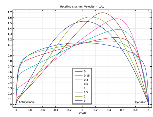
In the Settings window for 1D Plot Group, type Rotating channel: velocity profiles in the Label text field.
3
Locate the Data section. From the Parameter selection (Ro) list, choose From list.
4
In the Parameter values (Ro) list, choose 0, 0.15, 0.3, 0.6, 1, 1.5, 2, and 3.
5
Click to expand the Title section. From the Title type list, choose Manual.
6
In the Title text area, type Rotating channel: Velocity - u/U<sub>b</sub>.
7
Locate the Plot Settings section.
8
Select the x-axis label checkbox. In the associated text field, type 2*y/H.
9
Select the y-axis label checkbox.
10
Locate the Legend section. From the Position list, choose Lower middle.
Line Graph 1
1
Right-click Rotating channel: velocity profiles and choose Line Graph.
2
3
In the Settings window for Line Graph, locate the y-Axis Data section.
4
In the Expression text field, type u/U_i.
5
Locate the x-Axis Data section. From the Parameter list, choose Expression.
6
In the Expression text field, type 2*y/H.
7
Click to expand the Coloring and Style section. From the Color cycle list, choose Long.
8
Click to expand the Legends section. Select the Show legends checkbox.
Annotation 1
1
In the Model Builder window, right-click Rotating channel: velocity profiles and choose Annotation.
2
In the Settings window for Annotation, locate the Coloring and Style section.
3
From the Anchor point list, choose Lower left.
4
Locate the Position section. In the x text field, type -1.
5
Locate the Annotation section. In the Text text field, type Anticyclonic.
Annotation 2
1
Right-click Annotation 1 and choose Duplicate.
2
In the Settings window for Annotation, locate the Coloring and Style section.
3
From the Anchor point list, choose Lower right.
4
Locate the Position section. In the x text field, type 1.
5
Locate the Annotation section. In the Text text field, type Cyclonic.
Rotating channel: friction velocities
1
In the Results toolbar, click  1D Plot Group.
2
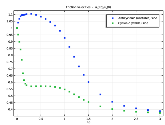
In the Settings window for 1D Plot Group, type Rotating channel: friction velocities in the Label text field.
3
Locate the Title section. From the Title type list, choose Manual.
4
In the Title text area, type Friction velocities - u<sub>\tau</sub>(Ro)/u<sub>\tau</sub>(0).
5
Locate the Plot Settings section.
6
Select the x-axis label checkbox. In the associated text field, type Ro.
7
Select the y-axis label checkbox.
Global 1
1
Right-click Rotating channel: friction velocities and choose Global.
2
In the Settings window for Global, locate the y-Axis Data section.
3
4
Click to expand the Coloring and Style section. Find the Line style subsection. From the Line list, choose None.
5
Find the Line markers subsection. From the Marker list, choose Point.
6
Click to expand the Legends section. From the Legends list, choose Manual.
7
Expanded section: friction coefficients
1
In the Results toolbar, click  1D Plot Group.
2
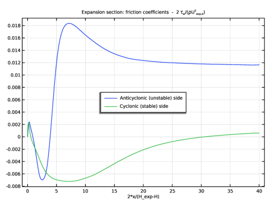
In the Settings window for 1D Plot Group, type Expanded section: friction coefficients in the Label text field.
3
Locate the Data section. From the Dataset list, choose Study 2/Solution 3 (sol3).
4
Locate the Title section. From the Title type list, choose Manual.
5
In the Title text area, type Expansion section: friction coefficients - 2 \tau<sub>w</sub>/(\rho U<sup>2</sup><sub>exp,b</sub>).
6
Locate the Plot Settings section.
7
Select the x-axis label checkbox. In the associated text field, type 2*x/(H_exp-H).
8
Select the y-axis label checkbox.
9
Locate the Legend section. From the Position list, choose Center.
Line Graph 1
1
Right-click Expanded section: friction coefficients and choose Line Graph.
2
3
In the Settings window for Line Graph, locate the y-Axis Data section.
4
In the Expression text field, type 2*spf2.nu*ppr(u2y)/(U_i*H/H_exp)^2.
5
Locate the x-Axis Data section. From the Parameter list, choose Expression.
6
In the Expression text field, type 4*x/H.
7
Locate the Legends section. Select the Show legends checkbox.
8
From the Legends list, choose Manual.
9
Line Graph 2
1
Right-click Line Graph 1 and choose Duplicate.
2
In the Settings window for Line Graph, locate the y-Axis Data section.
3
In the Expression text field, type -2*spf2.nu*ppr(u2y)/(U_i*H/H_exp)^2.
4
Locate the Selection section. Click  Clear Selection.
5
6
Locate the Legends section. In the table, enter the following settings:
Cut Line 2D 1
1
In the Results toolbar, click  Cut Line 2D.
2
In the Settings window for Cut Line 2D, locate the Data section.
3
From the Dataset list, choose Study 2/Solution 3 (sol3).
4
Locate the Line Data section. In row Point 1, set y to -H_exp/2.
5
In row Point 2, set x to 0.46.
6
In row Point 2, set y to -0.62.
Cut Line 2D 2
1
Right-click Cut Line 2D 1 and choose Duplicate.
2
In the Settings window for Cut Line 2D, locate the Line Data section.
3
In row Point 1, set y to H_exp/2.
4
In row Point 2, set x to 1.27.
5
In row Point 2, set y to 0.58.
Velocity and streamlines (spf2)
1
In the Model Builder window, under Results click Velocity (spf2).
2
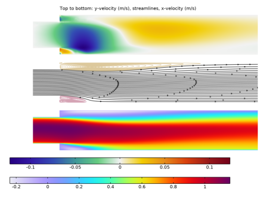
In the Settings window for 2D Plot Group, type Velocity and streamlines (spf2) in the Label text field.
3
Locate the Plot Settings section. From the View list, choose New view.
4
In the Velocity and streamlines (spf2) toolbar, click  Plot.
5
Click to expand the Title section. From the Title type list, choose Manual.
6
In the Title text area, type Top to bottom: y-velocity (m/s), streamlines, x-velocity (m/s).
7
Locate the Color Legend section. From the Position list, choose Bottom.
8
Locate the Plot Settings section. Clear the Plot dataset edges checkbox.
9
Click to expand the Plot Array section. From the Array type list, choose Linear.
10
From the Array axis list, choose y.
11
In the Relative padding text field, type 0.2.
Surface
1
In the Model Builder window, expand the Velocity and streamlines (spf2) node, then click Surface.
2
In the Settings window for Surface, locate the Expression section.
3
In the Expression text field, type v2.
4
Locate the Coloring and Style section. From the Color table list, choose Tectocoris.
5
Click to expand the Range section. Select the Manual color range checkbox.
6
In the Minimum text field, type -0.123.
7
In the Maximum text field, type 0.123.
8
Click to expand the Plot Array section. Select the Manual indexing checkbox.
9
In the Index text field, type 2.
Streamline 1
1
In the Model Builder window, right-click Velocity and streamlines (spf2) and choose Streamline.
2
In the Settings window for Streamline, locate the Expression section.
3
In the x-component text field, type u2.
4
In the y-component text field, type v2.
5
Locate the Streamline Positioning section. In the Number text field, type 25.
6
7
Locate the Coloring and Style section. Find the Point style subsection. From the Type list, choose Arrow.
8
From the Arrow distribution list, choose Equal time.
9
Click to expand the Advanced section. In the Loop tolerance text field, type 0.003.
10
Click to expand the Plot Array section. Select the Manual indexing checkbox.
11
In the Index text field, type 1.
Streamline 2
1
Right-click Streamline 1 and choose Duplicate.
2
In the Settings window for Streamline, locate the Streamline Positioning section.
3
From the Positioning list, choose Starting-point controlled.
4
From the Along curve list, choose Cut Line 2D 1.
5
Locate the Coloring and Style section. Find the Point style subsection. From the Type list, choose None.
6
From the Color list, choose Custom.
7
8
Click Define custom colors.
9
10
Click Add to custom colors.
11
Click Show color palette only or OK on the cross-platform desktop.
Streamline 3
1
Right-click Streamline 2 and choose Duplicate.
2
In the Settings window for Streamline, locate the Streamline Positioning section.
3
From the Along curve list, choose Cut Line 2D 2.
4
Locate the Coloring and Style section. Click Define custom colors.
5
6
Click Add to custom colors.
7
Click Show color palette only or OK on the cross-platform desktop.
Surface 2
1
In the Model Builder window, right-click Surface and choose Duplicate.
2
In the Settings window for Surface, locate the Expression section.
3
In the Expression text field, type u2.
4
Locate the Coloring and Style section. From the Color table list, choose Prism.
5
Locate the Range section. In the Minimum text field, type -0.24.
6
In the Maximum text field, type 1.16.
7
Locate the Plot Array section. In the Index text field, type 0.
8
In the Velocity and streamlines (spf2) toolbar, click  Plot.
Pressure and velocity (spf2)
1
In the Model Builder window, under Results click Pressure (spf2).
2
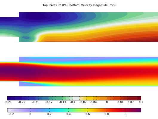
In the Settings window for 2D Plot Group, type Pressure and velocity (spf2) in the Label text field.
3
Locate the Plot Settings section. From the View list, choose New view.
4
In the Pressure and velocity (spf2) toolbar, click  Plot.
5
Locate the Title section. From the Title type list, choose Manual.
6
In the Title text area, type Top: Pressure (Pa); Bottom: Velocity magnitude (m/s).
7
Locate the Plot Array section. From the Array type list, choose Linear.
8
From the Array axis list, choose y.
9
In the Relative padding text field, type 0.5.
10
Locate the Plot Settings section. Clear the Plot dataset edges checkbox.
11
Locate the Color Legend section. From the Position list, choose Bottom.
Surface 2
Right-click Pressure and velocity (spf2) and choose Surface.
Surface 1
1
In the Settings window for Surface, locate the Coloring and Style section.
2
In the Number of bands text field, type 30.
3
Locate the Plot Array section. Select the Manual indexing checkbox.
4
In the Index text field, type 1.
Surface 2
1
In the Model Builder window, click Surface 2.
2
In the Settings window for Surface, locate the Expression section.
3
In the Expression text field, type spf2.U.
4
Locate the Coloring and Style section. From the Color table list, choose Prism.
5
Locate the Range section. Select the Manual color range checkbox.
6
In the Minimum text field, type -0.24.
7
In the Maximum text field, type 1.16.
8
Locate the Plot Array section. Select the Manual indexing checkbox.
9
In the Pressure and velocity (spf2) toolbar, click  Plot.
Reynolds stresses
1
In the Results toolbar, click  2D Plot Group.
2
In the Settings window for 2D Plot Group, type Reynolds stresses in the Label text field.
3
Locate the Data section. From the Dataset list, choose Study 2/Solution 3 (sol3).
4
Locate the Title section. From the Title type list, choose Manual.
5
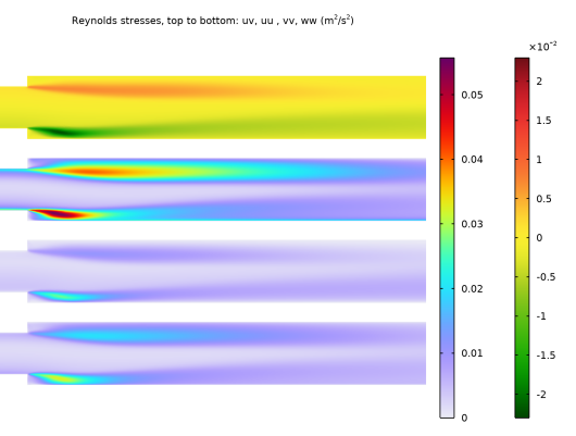
In the Title text area, type Reynolds stresses, top to bottom: uv, uu , vv, ww (m<sup>2</sup>/s<sup>2</sup>).
6
Clear the Parameter indicator text field.
7
Locate the Plot Settings section. Clear the Plot dataset edges checkbox.
8
Locate the Plot Array section. From the Array type list, choose Linear.
9
From the Array axis list, choose y.
Surface 1
1
Right-click Reynolds stresses and choose Surface.
2
In the Settings window for Surface, locate the Expression section.
3
In the Expression text field, type ww2.
4
Locate the Coloring and Style section. From the Color table list, choose Prism.
Surface 2
1
Right-click Surface 1 and choose Duplicate.
2
In the Settings window for Surface, locate the Expression section.
3
In the Expression text field, type vv2.
4
Click to expand the Inherit Style section. From the Plot list, choose Surface 1.
Surface 3
1
Right-click Surface 2 and choose Duplicate.
2
In the Settings window for Surface, locate the Expression section.
3
In the Expression text field, type uu2.
Surface 4
1
In the Model Builder window, under Results > Reynolds stresses right-click Surface 1 and choose Duplicate.
2
In the Settings window for Surface, locate the Expression section.
3
In the Expression text field, type uv2.
4
Locate the Coloring and Style section. From the Color table list, choose Traffic.
5
Locate the Range section. Select the Manual color range checkbox.
6
In the Minimum text field, type -0.023.
7
In the Maximum text field, type 0.023.
8
In the Reynolds stresses toolbar, click  Plot.