
|
|
|

|
1
|
|
2
|
In the Select Physics tree, select Fluid Flow > Single-Phase Flow > Turbulent Flow > Turbulent Flow, SSG-LRR (spf).
|
|
3
|
Click Add.
|
|
4
|
Click Add.
|
|
5
|
Click
|
|
6
|
In the Select Study tree, select Preset Studies for Selected Physics Interfaces > Stationary with Initialization.
|
|
7
|
Click
|
|
1
|
|
2
|
|
3
|
|
4
|
Browse to the model’s Application Libraries folder and double-click the file rotating_pipe_swirling_jet_parameters_1.txt.
|
|
1
|
|
2
|
|
3
|
|
4
|
Browse to the model’s Application Libraries folder and double-click the file rotating_pipe_swirling_jet_parameters_2.txt.
|
|
1
|
In the Model Builder window, under Component 1 (comp1) right-click Definitions and choose Variables.
|
|
2
|
|
1
|
Go to the Add Material window.
|
|
2
|
|
3
|
Click the Add to Component button in the window toolbar.
|
|
4
|
|
1
|
|
2
|
|
3
|
|
4
|
|
5
|
|
6
|
Click to expand the Layers section. In the table, enter the following settings:
|
|
1
|
|
2
|
|
3
|
|
4
|
|
1
|
|
2
|
|
3
|
|
4
|
|
5
|
|
6
|
|
1
|
|
2
|
|
3
|
|
4
|
|
5
|
|
1
|
|
2
|
|
3
|
|
4
|
|
5
|
|
1
|
|
2
|
|
3
|
|
4
|
|
5
|
|
1
|
|
2
|
Select the object r4 only.
|
|
3
|
|
4
|
|
5
|
Select the object r5 only.
|
|
6
|
Select the Keep objects to subtract checkbox.
|
|
1
|
|
2
|
Select the object r6 only.
|
|
3
|
|
4
|
|
5
|
Select the object r5 only.
|
|
1
|
|
2
|
|
4
|
Click
|
|
1
|
|
1
|
|
2
|
|
3
|
|
4
|
|
5
|
Click OK.
|
|
1
|
|
2
|
|
3
|
Click
|
|
5
|
|
1
|
In the Model Builder window, under Component 1 (comp1) > Turbulent Flow, SSG-LRR (spf) click Fluid Properties 1.
|
|
2
|
|
3
|
|
4
|
|
1
|
|
2
|
|
3
|
Specify the u vector as
|
|
1
|
|
2
|
|
3
|
|
4
|
|
1
|
|
3
|
|
4
|
|
5
|
|
1
|
|
1
|
|
2
|
|
3
|
|
1
|
|
3
|
|
4
|
|
5
|
|
6
|
|
7
|
|
1
|
|
3
|
|
4
|
|
5
|
Click
|
|
1
|
|
2
|
In the Settings window for Wall Distance Initialization, locate the Physics and Variables Selection section.
|
|
3
|
In the Solve for column of the table, under Component 1 (comp1), clear the checkbox for Turbulent Flow, SSG-LRR 2 (spf2).
|
|
1
|
|
2
|
|
3
|
In the Solve for column of the table, under Component 1 (comp1), clear the checkbox for Turbulent Flow, SSG-LRR 2 (spf2).
|
|
4
|
|
5
|
Click
|
|
1
|
|
2
|
In the Model Builder window, expand the Solution 1 (sol1) node, then click Compile Equations: Wall Distance Initialization.
|
|
3
|
|
4
|
|
5
|
|
6
|
|
7
|
Click OK.
|
|
8
|
|
1
|
|
3
|
|
4
|
Select the Swirl flow checkbox.
|
|
1
|
In the Model Builder window, under Component 1 (comp1) > Turbulent Flow, SSG-LRR 2 (spf2) click Fluid Properties 1.
|
|
2
|
|
3
|
|
4
|
|
1
|
|
2
|
|
3
|
Specify the u vector as
|
|
1
|
|
3
|
|
4
|
Click the Velocity field button.
|
|
5
|
|
6
|
|
7
|
From the list, choose Symmetric.
|
|
8
|
|
9
|
|
1
|
|
3
|
|
4
|
|
1
|
|
3
|
|
4
|
|
5
|
|
1
|
|
3
|
|
4
|
|
1
|
|
3
|
|
4
|
Clear the Suppress backflow checkbox.
|
|
1
|
|
2
|
|
1
|
|
3
|
|
4
|
|
5
|
|
6
|
|
7
|
|
8
|
Select the Reverse direction checkbox.
|
|
1
|
|
2
|
|
3
|
|
1
|
|
3
|
|
4
|
|
5
|
|
6
|
|
7
|
|
1
|
|
3
|
|
4
|
|
5
|
|
6
|
|
7
|
|
8
|
Select the Reverse direction checkbox.
|
|
1
|
|
3
|
|
4
|
|
5
|
|
6
|
|
7
|
|
1
|
|
2
|
|
3
|
|
1
|
|
2
|
|
3
|
Click
|
|
5
|
|
6
|
|
1
|
|
2
|
|
3
|
|
5
|
|
6
|
|
1
|
|
2
|
|
3
|
Click
|
|
5
|
|
6
|
|
1
|
|
2
|
|
3
|
|
1
|
|
2
|
|
3
|
|
4
|
|
5
|
Click the Custom button.
|
|
6
|
Locate the Element Size Parameters section.
|
|
7
|
|
1
|
|
2
|
|
3
|
|
5
|
|
6
|
Click the Custom button.
|
|
7
|
Click the Predefined button.
|
|
8
|
|
9
|
Click the Custom button.
|
|
10
|
Locate the Element Size Parameters section.
|
|
11
|
|
1
|
|
2
|
|
3
|
|
1
|
|
2
|
|
3
|
Click
|
|
5
|
|
6
|
|
1
|
|
2
|
|
3
|
|
5
|
|
6
|
Locate the Element Size Parameters section.
|
|
7
|
|
1
|
|
3
|
|
4
|
|
5
|
|
6
|
Click the Custom button.
|
|
7
|
Locate the Element Size Parameters section.
|
|
8
|
|
1
|
|
2
|
|
3
|
|
5
|
|
6
|
Click the Custom button.
|
|
7
|
Locate the Element Size Parameters section.
|
|
8
|
|
1
|
|
2
|
|
3
|
|
1
|
|
3
|
|
4
|
|
5
|
Click
|
|
1
|
|
2
|
Go to the Add Study window.
|
|
3
|
Find the Studies subsection. In the Select Study tree, select Preset Studies for Selected Physics Interfaces > Stationary with Initialization.
|
|
4
|
Click the Add Study button in the window toolbar.
|
|
5
|
|
1
|
In the Settings window for Wall Distance Initialization, locate the Physics and Variables Selection section.
|
|
2
|
In the Solve for column of the table, under Component 1 (comp1), clear the checkbox for Turbulent Flow, SSG-LRR (spf).
|
|
1
|
|
2
|
|
3
|
In the Solve for column of the table, under Component 1 (comp1), clear the checkbox for Turbulent Flow, SSG-LRR (spf).
|
|
4
|
|
5
|
Click
|
|
1
|
|
2
|
In the Model Builder window, expand the Solution 3 (sol3) node, then click Compile Equations: Wall Distance Initialization.
|
|
3
|
|
4
|
|
5
|
|
6
|
|
7
|
Click OK.
|
|
8
|
|
1
|
|
2
|
|
3
|
Select the Only plot when requested checkbox.
|
|
1
|
|
2
|
|
1
|
|
3
|
|
4
|
|
5
|
Locate the Expressions section. In the table, enter the following settings:
|
|
1
|
|
2
|
|
1
|
|
2
|
|
1
|
|
2
|
|
4
|
|
1
|
Go to the Evaluation Group 1 window.
|
|
2
|
Click the Full Precision button in the window toolbar.
|
|
1
|
|
2
|
|
1
|
|
2
|
|
3
|
|
4
|
|
1
|
|
1
|
|
2
|
|
3
|
|
4
|
|
5
|
|
1
|
|
2
|
|
1
|
|
2
|
|
3
|
|
1
|
|
2
|
|
3
|
|
4
|
|
5
|
|
6
|
|
7
|
|
1
|
|
2
|
|
3
|
|
4
|
|
5
|
|
6
|
|
1
|
|
2
|
|
3
|
Select the Scale checkbox.
|
|
4
|
|
1
|
|
2
|
|
3
|
|
4
|
|
5
|
Select the Additional parallel lines checkbox.
|
|
6
|
|
1
|
|
2
|
|
3
|
|
1
|
In the Model Builder window, under Results > Datasets right-click Revolution 2D 1 and choose Duplicate.
|
|
2
|
|
3
|
|
4
|
|
1
|
|
2
|
|
3
|
|
4
|
|
5
|
|
6
|
|
7
|
Locate the Plot Settings section.
|
|
8
|
|
9
|
Select the y-axis label checkbox. Clear the associated text field.
|
|
10
|
|
1
|
|
3
|
|
4
|
|
5
|
|
6
|
|
7
|
Click to expand the Coloring and Style section. Find the Line style subsection. From the Line list, choose Cycle.
|
|
8
|
|
9
|
|
10
|
|
12
|
|
1
|
|
2
|
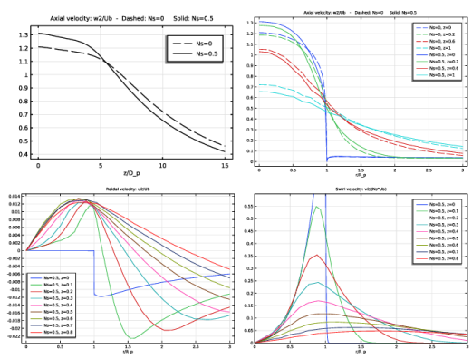
In the Settings window for 1D Plot Group, type Rotating Pipe Tangential Velocity in the Label text field.
|
|
3
|
|
4
|
|
5
|
|
6
|
|
7
|
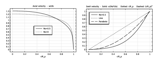
In the Title text area, type Swirl velocity - Solid: v/(Ns*Ub) Dotted: r/R_p Dashed: (r/R_p)<sup>2</sup>.
|
|
8
|
Locate the Plot Settings section.
|
|
9
|
|
1
|
|
3
|
|
4
|
|
5
|
|
6
|
|
7
|
|
8
|
|
10
|
Locate the Coloring and Style section. Find the Line style subsection. From the Line list, choose Cycle.
|
|
11
|
|
1
|
|
2
|
|
3
|
|
4
|
Locate the Legends section. In the table, enter the following settings:
|
|
1
|
|
2
|
|
3
|
|
4
|
Locate the Legends section. In the table, enter the following settings:
|
|
1
|
|
2
|
|
3
|
|
4
|
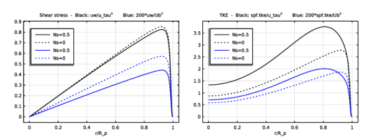
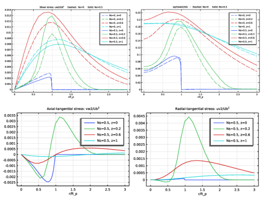
In the Title text area, type Shear stress - Black: uw/u_tau<sup>2</sup> Blue: 200*uw/Ub<sup>2</sup>.
|
|
5
|
Locate the Plot Settings section.
|
|
6
|
|
1
|
|
2
|
|
3
|
|
1
|
|
2
|
|
3
|
|
4
|
Click to expand the Coloring and Style section. Find the Line style subsection. From the Line list, choose Cycle (reset).
|
|
5
|
|
1
|
|
2
|
|
3
|
|
1
|
|
2
|
In the Settings window for 1D Plot Group, type Pipe Turbulence Kinetic Energy in the Label text field.
|
|
3
|
Locate the Title section. In the Title text area, type TKE - Black: spf.tke/u_tau<sup>2</sup> Blue: 200*spf.tke/Ub<sup>2</sup>.
|
|
1
|
In the Model Builder window, expand the Pipe Turbulence Kinetic Energy node, then click Line Graph 1.
|
|
2
|
|
3
|
|
1
|
|
2
|
|
3
|
|
1
|
|
2
|
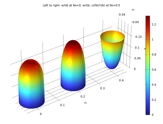
In the Settings window for 3D Plot Group, type Rotating Pipe 3D Velocity Profiles in the Label text field.
|
|
3
|
|
4
|
|
5
|
|
6
|
|
7
|
|
1
|
|
2
|
|
3
|
|
4
|
|
5
|
|
6
|
|
1
|
|
2
|
|
3
|
|
4
|
Locate the Scale section.
|
|
5
|
|
1
|
In the Model Builder window, under Results > Rotating Pipe 3D Velocity Profiles right-click Surface 1 and choose Duplicate.
|
|
2
|
|
3
|
|
4
|
|
1
|
|
2
|
Clear the Show axis orientation checkbox.
|
|
1
|
In the Model Builder window, expand the Results > Rotating Pipe 3D Velocity Profiles > Surface 3 node, then click Surface 3.
|
|
2
|
|
3
|
|
1
|
|
2
|
|
3
|
|
1
|
|
2
|
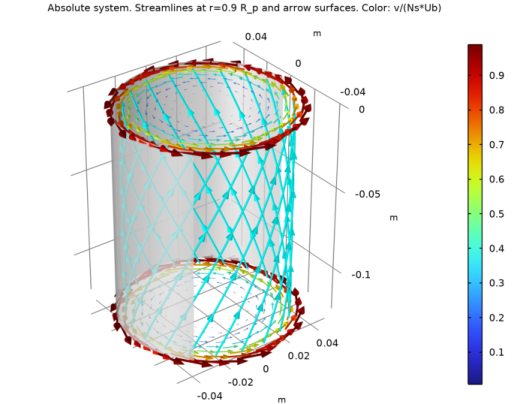
In the Settings window for 3D Plot Group, type Rotating Pipe Streamlines and Surface Arrows in the Label text field.
|
|
3
|
|
4
|
|
5
|
|
6
|
In the Title text area, type Absolute system. Streamlines at r=0.9 R_p and arrow surfaces. Color: v/(Ns*Ub).
|
|
1
|
|
2
|
|
3
|
|
4
|
|
5
|
|
6
|
Locate the Streamline Positioning section. From the Along curve or surface list, choose Parametric Curve 3D 1.
|
|
7
|
Locate the Coloring and Style section. Find the Line style subsection. From the Type list, choose Tube.
|
|
8
|
|
9
|
|
1
|
In the Model Builder window, right-click Rotating Pipe Streamlines and Surface Arrows and choose Arrow Surface.
|
|
2
|
|
3
|
|
4
|
|
5
|
|
6
|
|
7
|
Locate the Coloring and Style section.
|
|
8
|
|
1
|
|
2
|
|
3
|
|
1
|
In the Model Builder window, under Results > Rotating Pipe Streamlines and Surface Arrows right-click Arrow Surface 1 and choose Duplicate.
|
|
2
|
|
3
|
|
1
|
|
2
|
|
3
|
|
1
|
In the Model Builder window, right-click Rotating Pipe Streamlines and Surface Arrows and choose Surface.
|
|
2
|
|
3
|
|
4
|
|
5
|
|
6
|
|
1
|
|
2
|
|
3
|
Select the Scale checkbox.
|
|
4
|
|
1
|
|
2
|
|
3
|
|
1
|
|
2
|
|
3
|
Clear the Show axis orientation checkbox.
|
|
1
|
In the Model Builder window, right-click Rotating Pipe Streamlines and Surface Arrows and choose Duplicate.
|
|
2
|
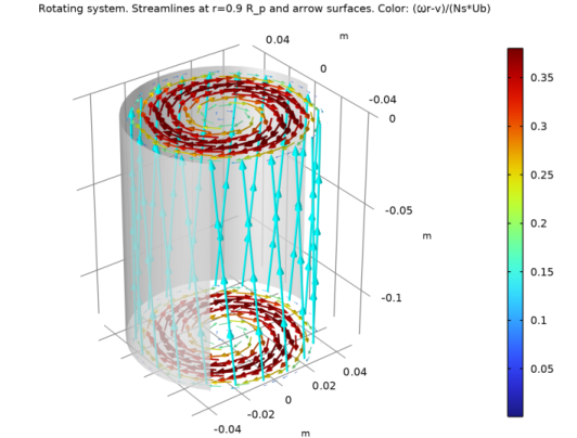
In the Settings window for 3D Plot Group, type Rotating Pipe Streamlines and Surface Arrows, Rotating Frame in the Label text field.
|
|
3
|
|
4
|
In the Title text area, type Rotating system. Streamlines at r=0.9 R_p and arrow surfaces. Color: (\omega r-v)/(Ns*Ub).
|
|
1
|
In the Model Builder window, expand the Rotating Pipe Streamlines and Surface Arrows, Rotating Frame node, then click Streamline 1.
|
|
2
|
|
3
|
|
4
|
|
1
|
|
2
|
|
3
|
|
4
|
|
5
|
|
1
|
|
2
|
|
3
|
|
1
|
In the Model Builder window, expand the Results > Rotating Pipe Streamlines and Surface Arrows, Rotating Frame > Arrow Surface 2 node, then click Arrow Surface 2.
|
|
2
|
|
3
|
|
4
|
|
1
|
|
2
|
|
3
|
|
1
|
|
2
|
|
3
|
|
4
|
|
5
|
|
6
|
|
7
|
Select the y-axis label checkbox.
|
|
8
|
|
9
|
Clear the y-axis label text field.
|
|
1
|
|
2
|
|
3
|
|
4
|
|
5
|
|
6
|
|
7
|
|
8
|
|
9
|
Locate the Coloring and Style section. Find the Line style subsection. From the Line list, choose Dashed.
|
|
10
|
|
11
|
|
1
|
|
2
|
|
3
|
|
4
|
Locate the Coloring and Style section. Find the Line style subsection. From the Line list, choose Solid.
|
|
5
|
|
6
|
Locate the Legends section. In the table, enter the following settings:
|
|
1
|
|
2
|
In the Settings window for 1D Plot Group, type Swirling Jet Axial Velocity Fluctuations in the Label text field.
|
|
3
|
|
1
|
In the Model Builder window, expand the Swirling Jet Axial Velocity Fluctuations node, then click Line Graph 1.
|
|
2
|
|
3
|
|
1
|
|
2
|
|
3
|
|
1
|
|
2
|
In the Settings window for 1D Plot Group, type Swirling Jet Axial Velocity on the Axis in the Label text field.
|
|
3
|
|
4
|
|
5
|
Locate the Plot Settings section.
|
|
6
|
|
7
|
Select the y-axis label checkbox. Clear the associated text field.
|
|
8
|
|
1
|
|
2
|
|
3
|
|
4
|
|
5
|
|
7
|
|
8
|
|
9
|
|
10
|
Locate the Coloring and Style section. Find the Line style subsection. From the Line list, choose Dashed.
|
|
11
|
|
12
|
|
13
|
|
1
|
|
2
|
|
3
|
|
4
|
Locate the Coloring and Style section. Find the Line style subsection. From the Line list, choose Solid.
|
|
5
|
Locate the Legends section. In the table, enter the following settings:
|
|
1
|
|
2
|
In the Settings window for 1D Plot Group, type Swirling Jet Radial Velocity in the Label text field.
|
|
3
|
|
4
|
|
5
|
|
6
|
Select the y-axis label checkbox.
|
|
7
|
|
8
|
Clear the y-axis label text field.
|
|
9
|
|
10
|
|
11
|
|
1
|
|
2
|
|
3
|
|
4
|
|
5
|
|
6
|
|
7
|
|
8
|
|
1
|
|
2
|
|
3
|
|
1
|
|
2
|
|
3
|
|
4
|
|
5
|
|
6
|
|
7
|
|
8
|
|
9
|
|
10
|
|
1
|
|
2
|
|
3
|
|
1
|
|
2
|
|
3
|
Locate the Title section. In the Title text area, type Shear stress: uw2/Ub<sup>2</sup> Dashed: Ns=0 Solid: Ns=0.5.
|
|
1
|
|
2
|
|
3
|
|
1
|
|
2
|
|
3
|
|
1
|
|
2
|
In the Settings window for 1D Plot Group, type Swirling Jet Radial-Tangential Stress in the Label text field.
|
|
3
|
|
4
|
|
5
|
|
6
|
Select the y-axis label checkbox.
|
|
7
|
|
8
|
Clear the y-axis label text field.
|
|
9
|
|
10
|
|
11
|
|
1
|
|
2
|
|
3
|
|
4
|
|
5
|
|
6
|
|
7
|
|
1
|
In the Model Builder window, right-click Swirling Jet Radial-Tangential Stress and choose Duplicate.
|
|
2
|
In the Settings window for 1D Plot Group, type Swirling Jet Axial-Tangential Stress in the Label text field.
|
|
3
|
|
1
|
In the Model Builder window, expand the Swirling Jet Axial-Tangential Stress node, then click Line Graph 1.
|
|
2
|
|
3
|
|
1
|
|
2
|
|
3
|
|
4
|
|
5
|
|
6
|
|
7
|
|
8
|
Clear the Parameter indicator text field.
|
|
9
|
Click to collapse the Title section. Locate the Plot Settings section. Clear the Plot dataset edges checkbox.
|
|
1
|
|
2
|
Clear the Show grid checkbox.
|
|
3
|
Clear the Show axis orientation checkbox.
|
|
1
|
|
2
|
|
3
|
|
4
|
|
5
|
|
6
|
|
7
|
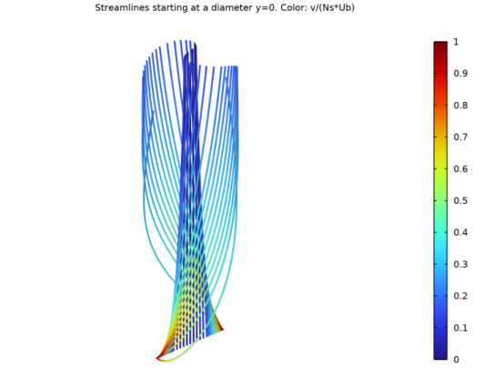
In the x text field, type range(-R_p,R_p/40,-3*R_p/4) range(-3*R_p/4,R_p/20,-R_p/2) range(-R_p/2,R_p/10,R_p/2) range(R_p/2,R_p/20,3*R_p/4) range(3*R_p/4,R_p/40,R_p).
|
|
8
|
|
9
|
|
10
|
Locate the Coloring and Style section. Find the Line style subsection. From the Type list, choose Tube.
|
|
11
|
|
12
|
|
13
|
|
14
|
Clear the Allow backward time integration checkbox.
|
|
1
|
|
2
|
|
3
|
 [
[