|
|
|
|
1
|
|
2
|
In the Select Physics tree, select Fluid Flow > High Mach Number Flow > Turbulent Flow > High Mach Number Flow, Low Reynolds Number k-ε (hmnf).
|
|
3
|
Click Add.
|
|
4
|
Click
|
|
5
|
In the Select Study tree, select Preset Studies for Selected Physics Interfaces > Stationary with Initialization.
|
|
6
|
Click
|
|
1
|
|
2
|
|
3
|
Click OK.
|
|
1
|
|
2
|
|
3
|
|
4
|
|
5
|
Click
|
|
6
|
Browse to the model’s Application Libraries folder and double-click the file rectangular_nozzle_parameters1.txt.
|
|
1
|
|
2
|
|
3
|
Click
|
|
4
|
Browse to the model’s Application Libraries folder and double-click the file rectangular_nozzle_parameters2.txt.
|
|
1
|
|
2
|
|
3
|
|
1
|
|
2
|
|
3
|
|
1
|
|
2
|
|
3
|
Select the View work plane geometry in 3D checkbox.
|
|
1
|
|
2
|
|
3
|
|
4
|
|
1
|
|
2
|
|
3
|
|
4
|
|
1
|
|
2
|
|
3
|
Click
|
|
4
|
Browse to the model’s Application Libraries folder and double-click the file rectangular_nozzle_polygon1.txt.
|
|
1
|
|
2
|
Select the object r1 only.
|
|
3
|
|
4
|
|
5
|
|
6
|
|
1
|
|
2
|
|
1
|
|
2
|
|
3
|
Select the View work plane geometry in 3D checkbox.
|
|
1
|
|
2
|
|
3
|
|
4
|
|
1
|
|
2
|
|
3
|
Click
|
|
4
|
Browse to the model’s Application Libraries folder and double-click the file rectangular_nozzle_polygon2.txt.
|
|
1
|
|
2
|
|
3
|
Click
|
|
4
|
Browse to the model’s Application Libraries folder and double-click the file rectangular_nozzle_polygon3.txt.
|
|
1
|
|
2
|
Select the object r1 only.
|
|
3
|
|
4
|
|
5
|
|
6
|
|
1
|
|
2
|
|
3
|
|
4
|
Select the object wp1 only.
|
|
5
|
Locate the Distances section. In the table, enter the following settings:
|
|
6
|
Select the Reverse direction checkbox.
|
|
1
|
|
2
|
|
3
|
Locate the Distances section. In the table, enter the following settings:
|
|
4
|
Click
|
|
1
|
|
2
|
Click in the Graphics window and then press Ctrl+A to select both objects.
|
|
3
|
|
4
|
|
5
|
|
6
|
Click OK.
|
|
1
|
|
2
|
|
3
|
|
4
|
On the object uni1, select Domains 4 and 5 only.
|
|
5
|
Click
|
|
1
|
|
2
|
|
3
|
|
4
|
|
5
|
|
6
|
|
7
|
Locate the Selections of Resulting Entities section. Find the Cumulative selection subsection. Click New.
|
|
8
|
|
9
|
Click OK.
|
|
1
|
|
2
|
In the Settings window for Work Plane, type Work Plane, Refinement Cross Section in the Label text field.
|
|
3
|
|
4
|
|
1
|
|
2
|
|
3
|
Select the View work plane geometry in 3D checkbox.
|
|
1
|
|
2
|
|
3
|
|
4
|
|
5
|
|
1
|
|
2
|
|
3
|
Locate the Distances section. In the table, enter the following settings:
|
|
4
|
Locate the Selections of Resulting Entities section. Find the Cumulative selection subsection. Click New.
|
|
5
|
|
6
|
Click OK.
|
|
1
|
|
2
|
|
3
|
|
4
|
|
5
|
|
1
|
|
2
|
In the Settings window for Work Plane, type Work Plane, Computational Cross Section in the Label text field.
|
|
3
|
|
1
|
|
2
|
|
3
|
|
4
|
|
1
|
|
2
|
|
3
|
Locate the Distances section. In the table, enter the following settings:
|
|
1
|
|
2
|
|
3
|
|
4
|
|
5
|
|
6
|
Click
|
|
1
|
|
2
|
|
3
|
|
4
|
|
1
|
|
2
|
On the object dif1, select Domain 2 only.
|
|
3
|
|
4
|
|
5
|
|
6
|
Clear the Automatic detection of small details checkbox.
|
|
1
|
|
2
|
|
3
|
|
4
|
|
1
|
|
2
|
|
3
|
|
1
|
|
2
|
|
3
|
|
1
|
|
2
|
|
3
|
|
4
|
|
1
|
|
2
|
|
3
|
|
4
|
|
5
|
|
6
|
Click OK.
|
|
7
|
|
8
|
|
9
|
|
10
|
Click OK.
|
|
1
|
|
2
|
|
3
|
|
1
|
|
2
|
|
3
|
|
4
|
|
5
|
In the Add dialog, in the Selections to invert list, choose Inlet, Co-Inlet, Outlet, No-Slip Wall, Coarse Mesh, No-Slip Wall, Fine Mesh, and Slip Wall.
|
|
6
|
Click OK.
|
|
1
|
|
2
|
|
1
|
|
2
|
|
1
|
|
2
|
|
3
|
|
4
|
|
5
|
Click OK.
|
|
1
|
|
2
|
|
3
|
|
1
|
|
2
|
|
3
|
|
4
|
|
5
|
Click OK.
|
|
1
|
|
2
|
|
3
|
|
1
|
|
2
|
|
1
|
|
2
|
|
3
|
|
4
|
Click
|
|
1
|
|
2
|
|
1
|
|
2
|
|
3
|
|
4
|
|
5
|
|
6
|
Click OK.
|
|
1
|
|
2
|
Go to the Add Material window.
|
|
3
|
|
4
|
Click the Add to Component button in the window toolbar.
|
|
5
|
|
1
|
In the Settings window for High Mach Number Flow, Low Reynolds Number k-ε, locate the Physical Model section.
|
|
2
|
|
3
|
Click to expand the Advanced Settings section.
|
|
1
|
In the Model Builder window, under Component 1 (comp1) > High Mach Number Flow, Low Reynolds Number k-ε (hmnf) click Fluid 1.
|
|
2
|
|
3
|
|
4
|
|
1
|
|
2
|
|
3
|
|
1
|
|
2
|
|
3
|
|
4
|
|
5
|
|
6
|
|
7
|
|
1
|
|
2
|
|
3
|
|
4
|
|
5
|
|
6
|
|
1
|
|
2
|
|
3
|
|
4
|
|
1
|
|
2
|
|
3
|
|
4
|
|
1
|
|
2
|
|
3
|
|
1
|
|
2
|
|
3
|
|
1
|
|
2
|
|
1
|
|
2
|
|
3
|
|
4
|
Locate the Geometric Entity Selection section. From the Geometric entity level list, choose Boundary.
|
|
5
|
|
6
|
|
1
|
|
2
|
|
3
|
|
4
|
|
5
|
|
6
|
|
7
|
Click the Custom button.
|
|
8
|
Locate the Element Size Parameters section.
|
|
9
|
|
1
|
|
2
|
|
3
|
|
4
|
|
5
|
|
6
|
|
7
|
Click the Custom button.
|
|
8
|
Locate the Element Size Parameters section.
|
|
9
|
|
1
|
|
2
|
|
3
|
|
1
|
|
2
|
In the Settings window for Boundary Layer Properties, locate the Geometric Entity Selection section.
|
|
3
|
|
4
|
|
1
|
|
2
|
|
3
|
|
4
|
|
1
|
|
2
|
|
3
|
Clear the Generate default plots checkbox.
|
|
1
|
|
2
|
|
3
|
Select the Auxiliary sweep checkbox.
|
|
4
|
Click
|
|
1
|
|
2
|
|
3
|
In the Model Builder window, expand the Study 1 > Solver Configurations > Solution 1 (sol1) > Stationary Solver 2 node, then click Segregated 1.
|
|
4
|
|
5
|
|
6
|
|
7
|
In the Model Builder window, expand the Study 1 > Solver Configurations > Solution 1 (sol1) > Stationary Solver 2 > AMG, fluid flow variables (hmnf) node, then click Multigrid 1.
|
|
8
|
|
9
|
|
10
|
In the Preconditioner variables list, choose Turbulent Dissipation Rate (comp1.ep), Reciprocal Wall Distance (comp1.G), Wall Temperature, Downside (comp1.hmnf.TWall_d), Wall Temperature, Upside (comp1.hmnf.TWall_u), Turbulent Kinetic Energy (comp1.k), and Temperature (comp1.T).
|
|
11
|
|
12
|
In the Model Builder window, under Study 1 > Solver Configurations > Solution 1 (sol1) > Stationary Solver 2 right-click AMG, fluid flow variables (hmnf) and choose Multigrid.
|
|
13
|
|
14
|
|
15
|
|
16
|
Select the Construct prolongators componentwise checkbox.
|
|
17
|
Clear the Prolongator smoothing checkbox.
|
|
18
|
Locate the Hybridization section. In the Preconditioner variables list, choose Turbulent Dissipation Rate (comp1.ep), Reciprocal Wall Distance (comp1.G), Turbulent Kinetic Energy (comp1.k), Pressure (comp1.p), and Velocity Field (comp1.u).
|
|
19
|
|
20
|
In the Model Builder window, expand the Study 1 > Solver Configurations > Solution 1 (sol1) > Stationary Solver 2 > AMG, fluid flow variables (hmnf) > Multigrid 2 > Presmoother node.
|
|
21
|
Right-click Study 1 > Solver Configurations > Solution 1 (sol1) > Stationary Solver 2 > AMG, fluid flow variables (hmnf) > Multigrid 2 > Presmoother and choose SOR Line.
|
|
22
|
|
23
|
|
24
|
|
25
|
|
26
|
|
27
|
|
28
|
In the Model Builder window, expand the Study 1 > Solver Configurations > Solution 1 (sol1) > Stationary Solver 2 > AMG, fluid flow variables (hmnf) > Multigrid 2 > Postsmoother node.
|
|
29
|
Right-click Study 1 > Solver Configurations > Solution 1 (sol1) > Stationary Solver 2 > AMG, fluid flow variables (hmnf) > Multigrid 2 > Postsmoother and choose SOR Line.
|
|
30
|
|
31
|
|
32
|
|
33
|
|
34
|
|
35
|
|
36
|
In the Model Builder window, expand the Study 1 > Solver Configurations > Solution 1 (sol1) > Stationary Solver 2 > AMG, fluid flow variables (hmnf) > Multigrid 2 > Coarse Solver node.
|
|
37
|
Right-click Study 1 > Solver Configurations > Solution 1 (sol1) > Stationary Solver 2 > AMG, fluid flow variables (hmnf) > Multigrid 2 > Coarse Solver and choose Direct.
|
|
38
|
|
39
|
|
40
|
|
41
|
|
1
|
In the Model Builder window, under Component 1 (comp1) right-click Definitions and choose Variables.
|
|
2
|
|
1
|
|
2
|
|
3
|
|
1
|
|
2
|
|
3
|
Click the Custom button.
|
|
4
|
Locate the Element Size Parameters section. In the Maximum element growth rate text field, type 1.1.
|
|
1
|
|
2
|
|
3
|
|
4
|
|
5
|
|
6
|
|
7
|
Click the Custom button.
|
|
8
|
Locate the Element Size Parameters section.
|
|
9
|
|
10
|
|
1
|
|
2
|
|
3
|
|
4
|
|
5
|
|
6
|
|
7
|
Click the Custom button.
|
|
8
|
Locate the Element Size Parameters section.
|
|
9
|
|
10
|
|
1
|
|
2
|
|
3
|
|
4
|
|
5
|
|
6
|
Click the Custom button.
|
|
7
|
Locate the Element Size Parameters section.
|
|
8
|
|
1
|
|
2
|
|
3
|
|
4
|
|
5
|
|
6
|
|
7
|
Click the Custom button.
|
|
8
|
Locate the Element Size Parameters section.
|
|
9
|
|
1
|
|
2
|
|
3
|
|
1
|
|
2
|
In the Settings window for Boundary Layer Properties, locate the Geometric Entity Selection section.
|
|
3
|
|
4
|
|
1
|
|
2
|
|
3
|
|
4
|
|
5
|
|
1
|
|
2
|
Go to the Add Study window.
|
|
3
|
Find the Studies subsection. In the Select Study tree, select Preset Studies for Selected Physics Interfaces > Stationary with Initialization.
|
|
4
|
Click the Add Study button in the window toolbar.
|
|
5
|
|
1
|
In the Settings window for Wall Distance Initialization, click to expand the Values of Dependent Variables section.
|
|
2
|
Find the Initial values of variables solved for subsection. From the Settings list, choose User controlled.
|
|
3
|
|
4
|
|
5
|
|
6
|
Find the Values of variables not solved for subsection. From the Settings list, choose User controlled.
|
|
7
|
|
8
|
|
9
|
|
1
|
|
2
|
|
3
|
|
4
|
|
5
|
Click
|
|
7
|
Find the Mesh adaptation subsection.
|
|
8
|
|
9
|
Locate the Geometric Entity Selection for Adaptation section. From the Geometric entity level list, choose Domain.
|
|
10
|
|
11
|
|
12
|
|
13
|
Select the Store complete solver history checkbox.
|
|
1
|
|
2
|
|
3
|
In the Model Builder window, expand the Study 2 > Solver Configurations > Solution 3 (sol3) > Stationary Solver 2 node, then click Adaptive Mesh Refinement.
|
|
4
|
|
5
|
Clear the Allow coarsening checkbox.
|
|
6
|
|
7
|
In the Model Builder window, under Study 2 > Solver Configurations > Solution 3 (sol3) > Stationary Solver 2 click Segregated 1.
|
|
8
|
|
9
|
|
10
|
|
11
|
|
12
|
|
13
|
|
14
|
|
15
|
|
16
|
Clear the Adaptive target error estimate checkbox.
|
|
17
|
|
18
|
In the Model Builder window, expand the Study 2 > Solver Configurations > Solution 3 (sol3) > Stationary Solver 2 > AMG, fluid flow variables (hmnf) node, then click Multigrid 1.
|
|
19
|
|
20
|
|
21
|
In the Preconditioner variables list, choose Turbulent Dissipation Rate (comp1.ep), Reciprocal Wall Distance (comp1.G), Wall Temperature, Downside (comp1.hmnf.TWall_d), Wall Temperature, Upside (comp1.hmnf.TWall_u), Turbulent Kinetic Energy (comp1.k), and Temperature (comp1.T).
|
|
22
|
|
23
|
In the Model Builder window, under Study 2 > Solver Configurations > Solution 3 (sol3) > Stationary Solver 2 right-click AMG, fluid flow variables (hmnf) and choose Multigrid.
|
|
24
|
|
25
|
|
26
|
|
27
|
Select the Construct prolongators componentwise checkbox.
|
|
28
|
Clear the Prolongator smoothing checkbox.
|
|
29
|
Locate the Hybridization section. In the Preconditioner variables list, choose Turbulent Dissipation Rate (comp1.ep), Reciprocal Wall Distance (comp1.G), Turbulent Kinetic Energy (comp1.k), Pressure (comp1.p), and Velocity Field (comp1.u).
|
|
30
|
|
31
|
In the Model Builder window, expand the Study 2 > Solver Configurations > Solution 3 (sol3) > Stationary Solver 2 > AMG, fluid flow variables (hmnf) > Multigrid 2 > Presmoother node.
|
|
32
|
Right-click Study 2 > Solver Configurations > Solution 3 (sol3) > Stationary Solver 2 > AMG, fluid flow variables (hmnf) > Multigrid 2 > Presmoother and choose SOR Line.
|
|
33
|
|
34
|
|
35
|
|
36
|
|
37
|
|
38
|
|
39
|
In the Model Builder window, expand the Study 2 > Solver Configurations > Solution 3 (sol3) > Stationary Solver 2 > AMG, fluid flow variables (hmnf) > Multigrid 2 > Postsmoother node.
|
|
40
|
Right-click Study 2 > Solver Configurations > Solution 3 (sol3) > Stationary Solver 2 > AMG, fluid flow variables (hmnf) > Multigrid 2 > Postsmoother and choose SOR Line.
|
|
41
|
|
42
|
|
43
|
|
44
|
|
45
|
|
46
|
|
47
|
In the Model Builder window, expand the Study 2 > Solver Configurations > Solution 3 (sol3) > Stationary Solver 2 > AMG, fluid flow variables (hmnf) > Multigrid 2 > Coarse Solver node.
|
|
48
|
Right-click Study 2 > Solver Configurations > Solution 3 (sol3) > Stationary Solver 2 > AMG, fluid flow variables (hmnf) > Multigrid 2 > Coarse Solver and choose Direct.
|
|
49
|
|
50
|
|
51
|
|
52
|
|
53
|
|
54
|
Clear the Generate default plots checkbox.
|
|
55
|
|
1
|
|
2
|
|
3
|
Select the Only plot when requested checkbox.
|
|
1
|
|
2
|
|
1
|
|
2
|
|
3
|
|
4
|
|
5
|
|
6
|
|
1
|
|
2
|
|
3
|
|
1
|
|
2
|
|
3
|
|
4
|
|
5
|
|
6
|
|
7
|
|
1
|
|
2
|
|
3
|
|
4
|
|
5
|
|
6
|
|
7
|
|
8
|
|
9
|
|
10
|
|
1
|
|
2
|
|
3
|
|
4
|
|
5
|
|
1
|
|
2
|
|
3
|
|
4
|
|
1
|
|
2
|
|
3
|
|
4
|
|
1
|
|
2
|
|
3
|
|
4
|
|
5
|
|
6
|
Select the Additional parallel lines checkbox.
|
|
7
|
|
1
|
|
2
|
|
3
|
|
4
|
|
5
|
|
6
|
|
7
|
Click
|
|
8
|
|
9
|
|
10
|
|
11
|
Click
|
|
1
|
|
2
|
|
3
|
|
4
|
Click
|
|
5
|
|
6
|
|
7
|
Click
|
|
1
|
|
2
|
|
3
|
|
4
|
|
5
|
Click
|
|
1
|
|
2
|
|
3
|
|
4
|
Click
|
|
5
|
|
6
|
Click
|
|
1
|
|
2
|
|
3
|
|
4
|
Click
|
|
5
|
|
6
|
Click
|
|
1
|
|
2
|
|
3
|
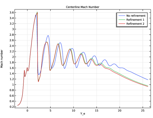
Locate the Data section. From the Dataset list, choose Study 2/Adaptive Mesh Refinement Solutions 1 (sol5).
|
|
4
|
|
5
|
Locate the Plot Settings section.
|
|
6
|
|
7
|
|
1
|
|
3
|
|
4
|
|
5
|
|
6
|
|
7
|
|
8
|
|
10
|
|
1
|
|
2
|
|
3
|
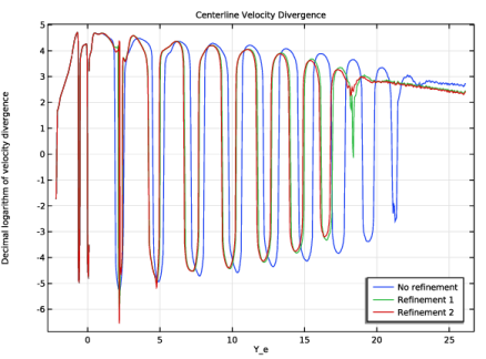
In the Settings window for 1D Plot Group, type Centerline Velocity Divergence in the Label text field.
|
|
4
|
Locate the Plot Settings section. In the y-axis label text field, type Decimal logarithm of velocity divergence.
|
|
5
|
|
1
|
|
2
|
|
3
|
|
4
|
|
1
|
|
2
|
|
3
|
|
1
|
|
2
|
|
3
|
|
4
|
|
5
|
|
1
|
|
2
|
In the Settings window for 3D Plot Group, type Jet Vertical-Horizontal Asymmetry in the Label text field.
|
|
3
|
|
4
|
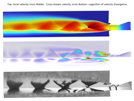
In the Title text area, type Top: Axial velocity (m/s) Middle: Cross-stream velocity (m/s) Bottom: Logarithm of velocity divergence.
|
|
5
|
Locate the Data section. From the Dataset list, choose Study 2/Adaptive Mesh Refinement Solutions 1 (sol5).
|
|
6
|
|
7
|
|
8
|
Clear the Plot dataset edges checkbox.
|
|
9
|
|
10
|
Clear the Show legends checkbox.
|
|
1
|
|
2
|
|
3
|
|
1
|
|
2
|
|
3
|
|
1
|
|
2
|
|
3
|
|
1
|
|
2
|
|
3
|
|
4
|
|
1
|
|
2
|
|
3
|
|
4
|
|
1
|
|
2
|
|
3
|
Locate the Expression section. In the Expression text field, type sign(hmnf.divu)*log10(abs(hmnf.divu)).
|
|
4
|
|
1
|
In the Model Builder window, expand the Compression-Expansion Strength node, then click Transformation 1.
|
|
2
|
|
3
|
|
4
|
|
5
|
|
6
|
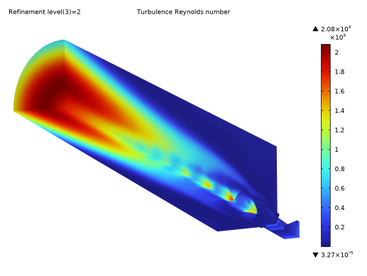
Adjust the camera to reproduce Figure 6.
|
|
1
|
|
2
|
|
3
|
Select the Show legends checkbox.
|
|
4
|
|
1
|
|
2
|
|
3
|
|
4
|
|
5
|
|
6
|
|
7
|
|
8
|
|
9
|
|
1
|
|
2
|
|
3
|
|
4
|
|
1
|
|
2
|
|
3
|
|
4
|
|
5
|
|
6
|
|
7
|
|
8
|
|
9
|
|
10
|
Select the Show maximum and minimum values checkbox.
|
|
1
|
|
2
|
|
3
|
|
4
|
|
1
|
|
2
|
|
3
|
Locate the Data section. From the Dataset list, choose Study 2/Adaptive Mesh Refinement Solutions 1 (sol5).
|
|
4
|
|
5
|
|
6
|
|
7
|
|
8
|
|
9
|
|
1
|
|
2
|
|
3
|
|
1
|
|
2
|
|
3
|
|
1
|
|
2
|
|
1
|
|
2
|
|
3
|
Locate the Data section. From the Dataset list, choose Study 2/Adaptive Mesh Refinement Solutions 1 (sol5).
|
|
4
|
|
5
|
|
6
|
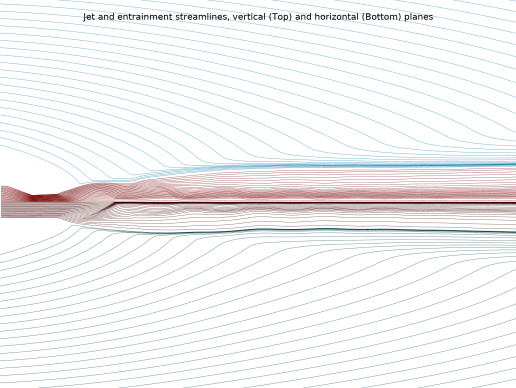
In the Title text area, type Jet and entrainment streamlines, vertical (Top) and horizontal (Bottom) planes.
|
|
7
|
|
8
|
|
1
|
|
2
|
In the Settings window for Streamline Surface, type Vertical Jet Streamlines in the Label text field.
|
|
3
|
|
4
|
|
5
|
|
6
|
|
7
|
|
8
|
Click OK.
|
|
9
|
|
10
|
|
11
|
|
12
|
|
13
|
|
14
|
Click Define custom colors.
|
|
16
|
Click Add to custom colors.
|
|
17
|
|
1
|
|
2
|
In the Settings window for Streamline Surface, type Vertical Entrainment Streamlines in the Label text field.
|
|
3
|
|
4
|
|
5
|
|
6
|
|
7
|
Click OK.
|
|
8
|
|
9
|
Click Define custom colors.
|
|
11
|
Click Add to custom colors.
|
|
12
|
|
1
|
|
2
|
In the Settings window for Streamline Surface, type Horizontal Jet Streamlines in the Label text field.
|
|
3
|
|
4
|
|
5
|
Click
|
|
6
|
|
7
|
Click OK.
|
|
8
|
|
9
|
Click Define custom colors.
|
|
11
|
Click Add to custom colors.
|
|
12
|
|
1
|
|
2
|
|
3
|
Clear the Move checkbox.
|
|
4
|
Select the Rotate checkbox.
|
|
5
|
|
6
|
|
1
|
|
2
|
In the Settings window for Streamline Surface, type Horizontal Entrainment Streamlines in the Label text field.
|
|
3
|
|
4
|
|
5
|
|
6
|
|
7
|
Click OK.
|
|
8
|
|
9
|
Click Define custom colors.
|
|
11
|
Click Add to custom colors.
|
|
12
|
|
13
|
|
1
|
|
2
|
In the Settings window for 2D Plot Group, type Jet Asymmetry Planar Perspective in the Label text field.
|
|
3
|
|
4
|
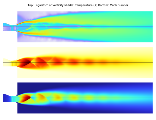
In the Title text area, type Top: Logarithm of vorticity Middle: Temperature (K) Bottom: Mach number.
|
|
5
|
|
6
|
|
1
|
|
2
|
|
3
|
|
1
|
|
2
|
|
3
|
|
1
|
|
2
|
|
3
|
|
4
|
|
1
|
|
2
|
|
3
|
Select the Scale checkbox.
|
|
4
|
|
1
|
|
2
|
|
3
|
|
4
|
|
1
|
|
2
|
|
3
|
|
1
|
|
2
|
|
3
|
|
4
|
|
1
|
|
2
|
|
3
|
|
1
|
|
2
|
In the Settings window for Surface, type Decimal Logarithm Vorticity Vertical Plane in the Label text field.
|
|
3
|
|
4
|
|
1
|
In the Model Builder window, expand the Decimal Logarithm Vorticity Vertical Plane node, then click Transformation 1.
|
|
2
|
|
3
|
|
1
|
|
2
|
In the Settings window for Surface, type Decimal Logarithm Vorticity Horizontal Plane in the Label text field.
|
|
3
|
|
4
|
Locate the Inherit Style section. From the Plot list, choose Decimal Logarithm Vorticity Vertical Plane.
|
|
1
|
In the Model Builder window, expand the Decimal Logarithm Vorticity Horizontal Plane node, then click Transformation 1.
|
|
2
|
|
3
|
|
1
|
|
2
|
|
3
|
|
4
|
|
5
|
|
6
|
|
7
|
|
8
|
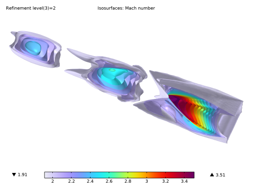
Adjust camera to reproduce Figure 7.
|
|
1
|
|
2
|
|
3
|
Select the Show legends checkbox.
|
|
1
|
|
2
|
|
3
|
|
4
|
|
1
|
|
3
|
|
1
|
|
2
|
|
3
|
|
1
|
|
3
|
|
5
|