
|
|
|

|
1
|
|
2
|
|
3
|
|
4
|
Browse to the model’s Application Libraries folder and double-click the file onera_m6_wing_geom_sequence.mph.
|
|
5
|
|
6
|
|
7
|
|
1
|
|
2
|
|
1
|
|
2
|
Go to the Add Material window.
|
|
3
|
|
4
|
Right-click and choose Add to Component 1 (comp1).
|
|
5
|
|
1
|
|
2
|
In the Settings window for Explicit, type Top and bottom surfaces of the wing in the Label text field.
|
|
3
|
|
4
|
Click
|
|
5
|
|
6
|
Click OK.
|
|
1
|
|
2
|
In the Settings window for Explicit, type Trailing edge surfaces of the wing in the Label text field.
|
|
3
|
|
4
|
Click
|
|
5
|
|
6
|
Click OK.
|
|
1
|
|
2
|
|
3
|
|
4
|
Click
|
|
5
|
|
6
|
Click OK.
|
|
1
|
|
2
|
|
3
|
|
4
|
|
5
|
In the Add dialog, in the Selections to add list, choose Top and bottom surfaces of the wing, Trailing edge surfaces of the wing, and Tip surfaces of the wing.
|
|
6
|
Click OK.
|
|
1
|
|
2
|
|
3
|
|
4
|
Click
|
|
5
|
|
6
|
Click OK.
|
|
1
|
|
2
|
|
3
|
|
4
|
Click
|
|
5
|
|
6
|
Click OK.
|
|
1
|
|
2
|
|
3
|
|
4
|
Click
|
|
5
|
|
6
|
Click OK.
|
|
1
|
|
2
|
|
3
|
|
4
|
Click
|
|
5
|
|
6
|
Click OK.
|
|
1
|
|
2
|
|
3
|
|
4
|
Click
|
|
5
|
|
6
|
Click OK.
|
|
1
|
|
2
|
|
3
|
|
4
|
Click
|
|
5
|
|
6
|
Click OK.
|
|
1
|
|
2
|
|
3
|
|
4
|
Click
|
|
5
|
|
6
|
Click OK.
|
|
1
|
|
2
|
|
3
|
From the list, choose User-controlled mesh.
|
|
1
|
|
2
|
|
3
|
Click
|
|
4
|
In the Paste Selection dialog, type 8, 9, 11, 12, 14, 15, 17, 18, 20, 21, 23, 24, 26, 27, 29, 30 in the Selection text field.
|
|
5
|
Click OK.
|
|
1
|
|
2
|
|
3
|
|
4
|
|
5
|
|
6
|
|
7
|
Select the Symmetric distribution checkbox.
|
|
1
|
|
2
|
|
3
|
Click
|
|
4
|
In the Paste Selection dialog, type 39, 41, 44, 46, 49, 51, 54, 56, 59, 61, 64, 66, 69, 71, 74, 76, 80, 82, 83 in the Selection text field.
|
|
5
|
Click OK.
|
|
1
|
|
2
|
|
3
|
|
1
|
|
2
|
|
3
|
Click
|
|
4
|
|
5
|
Click OK.
|
|
1
|
|
2
|
|
3
|
|
4
|
|
5
|
Click the Custom button.
|
|
6
|
Locate the Element Size Parameters section.
|
|
7
|
|
8
|
|
1
|
|
2
|
|
3
|
|
4
|
Click
|
|
5
|
|
6
|
Click OK.
|
|
7
|
|
8
|
|
1
|
|
2
|
|
3
|
|
4
|
Click
|
|
5
|
|
6
|
Click OK.
|
|
1
|
|
2
|
|
3
|
Click
|
|
4
|
|
5
|
Click OK.
|
|
1
|
|
2
|
|
3
|
|
4
|
|
5
|
Click the Custom button.
|
|
6
|
Locate the Element Size Parameters section.
|
|
7
|
|
8
|
|
1
|
|
2
|
|
3
|
|
4
|
|
5
|
Click the Custom button.
|
|
6
|
|
7
|
|
8
|
|
1
|
|
2
|
Drag and drop below Free Triangular 1.
|
|
3
|
|
1
|
|
2
|
Go to the Add Physics window.
|
|
3
|
In the tree, select Fluid Flow > High Mach Number Flow > Turbulent Flow > High Mach Number Flow, Spalart–Allmaras (hmnf).
|
|
4
|
Click the Add to Component 1 button in the window toolbar.
|
|
5
|
|
1
|
In the Model Builder window, under Component 1 (comp1) > High Mach Number Flow, Spalart–Allmaras (hmnf) click Initial Values 1.
|
|
2
|
|
3
|
Specify the u vector as
|
|
1
|
|
2
|
|
3
|
Click
|
|
4
|
|
5
|
Click OK.
|
|
1
|
|
2
|
|
3
|
Click
|
|
4
|
|
5
|
Click OK.
|
|
6
|
|
7
|
|
8
|
|
1
|
|
2
|
|
3
|
Click
|
|
4
|
|
5
|
Click OK.
|
|
1
|
|
2
|
Go to the Add Study window.
|
|
3
|
Find the Studies subsection. In the Select Study tree, select Preset Studies for Selected Physics Interfaces > Stationary with Initialization.
|
|
4
|
Click the Add Study button in the window toolbar.
|
|
5
|
|
1
|
|
2
|
|
3
|
Select the Auxiliary sweep checkbox.
|
|
4
|
Click
|
|
6
|
|
7
|
|
8
|
Clear the Generate default plots checkbox.
|
|
9
|
|
1
|
|
2
|
|
1
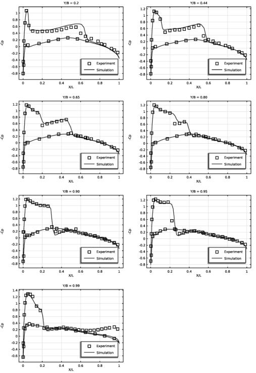
|
In the Settings window for Table, type Experimental Cp values along the top edge of the wing at Y/B = 0.20 in the Label text field.
|
|
2
|
|
3
|
Browse to the model’s Application Libraries folder and double-click the file onera_m6_wing_Cp_YbyB_1_up.txt.
|
|
1
|
|
2
|
In the Settings window for Table, type Experimental Cp values along the bottom edge of the wing at Y/B = 0.20 in the Label text field.
|
|
3
|
|
4
|
Browse to the model’s Application Libraries folder and double-click the file onera_m6_wing_Cp_YbyB_1_down.txt.
|
|
1
|
|
2
|
In the Settings window for Table, type Experimental Cp values along the top edge of the wing at Y/B = 0.44 in the Label text field.
|
|
3
|
|
4
|
Browse to the model’s Application Libraries folder and double-click the file onera_m6_wing_Cp_YbyB_2_up.txt.
|
|
1
|
|
2
|
In the Settings window for Table, type Experimental Cp values along the bottom edge of the wing at Y/B = 0.44 in the Label text field.
|
|
3
|
|
4
|
Browse to the model’s Application Libraries folder and double-click the file onera_m6_wing_Cp_YbyB_2_down.txt.
|
|
1
|
|
2
|
In the Settings window for Table, type Experimental Cp values along the top edge of the wing at Y/B = 0.65 in the Label text field.
|
|
3
|
|
4
|
Browse to the model’s Application Libraries folder and double-click the file onera_m6_wing_Cp_YbyB_3_up.txt.
|
|
1
|
|
2
|
In the Settings window for Table, type Experimental Cp values along the bottom edge of the wing at Y/B = 0.65 in the Label text field.
|
|
3
|
|
4
|
Browse to the model’s Application Libraries folder and double-click the file onera_m6_wing_Cp_YbyB_3_down.txt.
|
|
1
|
|
2
|
In the Settings window for Table, type Experimental Cp values along the top edge of the wing at Y/B = 0.80 in the Label text field.
|
|
3
|
|
4
|
Browse to the model’s Application Libraries folder and double-click the file onera_m6_wing_Cp_YbyB_4_up.txt.
|
|
1
|
|
2
|
In the Settings window for Table, type Experimental Cp values along the bottom edge of the wing at Y/B = 0.80 in the Label text field.
|
|
3
|
|
4
|
Browse to the model’s Application Libraries folder and double-click the file onera_m6_wing_Cp_YbyB_4_down.txt.
|
|
1
|
|
2
|
In the Settings window for Table, type Experimental Cp values along the top edge of the wing at Y/B = 0.90 in the Label text field.
|
|
3
|
|
4
|
Browse to the model’s Application Libraries folder and double-click the file onera_m6_wing_Cp_YbyB_5_up.txt.
|
|
1
|
|
2
|
In the Settings window for Table, type Experimental Cp values along the bottom edge of the wing at Y/B = 0.90 in the Label text field.
|
|
3
|
|
4
|
Browse to the model’s Application Libraries folder and double-click the file onera_m6_wing_Cp_YbyB_5_down.txt.
|
|
1
|
|
2
|
In the Settings window for Table, type Experimental Cp values along the top edge of the wing at Y/B = 0.95 in the Label text field.
|
|
3
|
|
4
|
Browse to the model’s Application Libraries folder and double-click the file onera_m6_wing_Cp_YbyB_6_up.txt.
|
|
1
|
|
2
|
In the Settings window for Table, type Experimental Cp values along the bottom edge of the wing at Y/B = 0.95 in the Label text field.
|
|
3
|
|
4
|
Browse to the model’s Application Libraries folder and double-click the file onera_m6_wing_Cp_YbyB_6_down.txt.
|
|
1
|
|
2
|
In the Settings window for Table, type Experimental Cp values along the top edge of the wing at Y/B = 0.99 in the Label text field.
|
|
3
|
|
4
|
Browse to the model’s Application Libraries folder and double-click the file onera_m6_wing_Cp_YbyB_7_up.txt.
|
|
1
|
|
2
|
In the Settings window for Table, type Experimental Cp values along the bottom edge of the wing at Y/B = 0.99 in the Label text field.
|
|
3
|
|
4
|
Browse to the model’s Application Libraries folder and double-click the file onera_m6_wing_Cp_YbyB_7_down.txt.
|
|
1
|
|
2
|
|
3
|
|
4
|
|
5
|
|
6
|
Locate the Plot Settings section.
|
|
7
|
|
8
|
|
9
|
|
1
|
|
2
|
|
3
|
|
4
|
|
5
|
|
6
|
|
7
|
|
1
|
|
2
|
|
3
|
|
4
|
Locate the Coloring and Style section. Find the Line markers subsection. From the Marker list, choose Square.
|
|
5
|
|
1
|
|
2
|
|
3
|
|
4
|
Locate the y-Axis Data section. In the Expression text field, type (1[atm] - hmnf.pA)/(0.5*hmnf.gamma*M_INF^2*1[atm]).
|
|
5
|
|
6
|
|
7
|
|
8
|
|
9
|
|
1
|
|
2
|
|
3
|
|
1
|
|
2
|
|
3
|
|
1
|
|
2
|
|
3
|
|
1
|
|
2
|
|
3
|
|
4
|
Locate the x-Axis Data section. In the Expression text field, type (x-0.30346[m])/(0.95700[m]-0.30346[m]).
|
|
1
|
|
2
|
|
3
|
|
1
|
|
2
|
|
3
|
|
1
|
|
2
|
|
3
|
|
1
|
|
2
|
|
3
|
|
4
|
Locate the x-Axis Data section. In the Expression text field, type (x-0.44829[m])/(1.0275[m]-0.44829[m]).
|
|
1
|
|
2
|
|
3
|
|
1
|
|
2
|
|
3
|
|
1
|
|
2
|
|
3
|
|
1
|
|
2
|
|
3
|
|
4
|
Locate the x-Axis Data section. In the Expression text field, type (x-0.55174[m])/(1.0778[m]-0.55174[m]).
|
|
1
|
|
2
|
|
3
|
|
1
|
|
2
|
|
3
|
|
1
|
|
2
|
|
3
|
|
1
|
|
2
|
|
3
|
|
4
|
Locate the x-Axis Data section. In the Expression text field, type (x-0.62070[m])/(1.1114[m]-0.62070[m]).
|
|
1
|
|
2
|
|
3
|
|
1
|
|
2
|
|
3
|
|
1
|
|
2
|
|
3
|
|
1
|
|
2
|
|
3
|
|
4
|
Locate the x-Axis Data section. In the Expression text field, type (x-0.65519[m])/(1.1282[m]-0.65519[m]).
|
|
1
|
|
2
|
|
3
|
|
1
|
|
2
|
|
3
|
|
1
|
|
2
|
|
3
|
|
1
|
|
2
|
|
3
|
|
4
|
Locate the x-Axis Data section. In the Expression text field, type (x-0.68277[m])/(1.1416[m]-0.68277[m]).
|
|
1
|
|
2
|
|
3
|
|
4
|
|
1
|
|
2
|
|
3
|
|
4
|
|
5
|
|
1
|
|
2
|
|
3
|
Click
|
|
4
|
In the Paste Selection dialog, type 6, 8, 10, 12, 14, 16, 18, 20, 22, 24, 26, 28, 30, 32, 34, 36, 38, 40, 42 in the Selection text field.
|
|
5
|
Click OK.
|
|
1
|
|
2
|
|
3
|
|
4
|
|
5
|
|
1
|
|
2
|
|
3
|
|
4
|
|
5
|
|
6
|
|
7
|
|
1
|
|
2
|
|
3
|
Click
|
|
4
|
In the Paste Selection dialog, type 6, 8, 10, 12, 14, 16, 18, 20, 22, 24, 26, 28, 30, 32, 34, 36, 38, 40, 42 in the Selection text field.
|
|
5
|
Click OK.
|
|
1
|
|
2
|
|
3
|
|
4
|
|
1
|
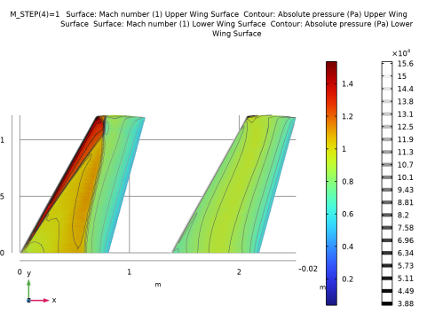
In the Model Builder window, under Results > Mach Number and Pressure right-click Surface 1 and choose Duplicate.
|
|
2
|
|
3
|
|
4
|
|
5
|
Click to expand the Plot Array section.
|
|
1
|
|
2
|
|
3
|
Click
|
|
4
|
Click
|
|
5
|
In the Paste Selection dialog, type 5, 7, 9, 11, 13, 15, 17, 19, 21, 23, 25, 27, 29, 31, 33, 35, 37, 39, 41 in the Selection text field.
|
|
6
|
Click OK.
|
|
1
|
In the Model Builder window, under Results > Mach Number and Pressure right-click Contour 1 and choose Duplicate.
|
|
2
|
|
3
|
|
4
|
|
5
|
|
6
|
|
1
|
|
2
|
|
3
|
Click
|
|
4
|
Click
|
|
5
|
In the Paste Selection dialog, type 5, 7, 9, 11, 13, 15, 17, 19, 21, 23, 25, 27, 29, 31, 33, 35, 37, 39, 41 in the Selection text field.
|
|
6
|
Click OK.
|
|
1
|
|
2
|
|
3
|
|
1
|
|
2
|
|
3
|
|
1
|
|
2
|
|
3
|
|
1
|
|
2
|
|
3
|
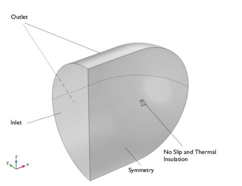
In the Logical expression for inclusion text field, type (x>-2*C0) && (x<3*C0) && (y<B+2*C0) && (z>-2*C0) && (z<2*C0).
|
|
1
|
|
2
|
|
3
|
|
4
|
|
5
|
|
6
|
Clear the Color legend checkbox.
|
|
1
|
|
2
|
|
3
|
|
1
|
|
2
|
|
3
|
Select the Use the plot’s color checkbox.
|
|
4
|
|
1
|
|
2
|
|
3
|
|
4
|
|
1
|
|
2
|
Click
|
|
1
|
|
2
|
|
1
|
|
2
|
|
3
|
|
1
|
|
2
|
|
3
|
|
1
|
|
2
|
|
3
|
|
4
|
|
5
|
|
6
|
|
1
|
In the Model Builder window, under Component 1 (comp1) > Geometry 1 right-click Work Plane 1 (wp1) and choose Revolve.
|
|
2
|
|
3
|
Click the Angles button.
|
|
4
|
|
5
|
Locate the Revolution Axis section. Find the Point on the revolution axis subsection. In the xw text field, type -C0/2.
|
|
1
|
|
2
|
|
3
|
|
4
|
|
1
|
|
2
|
|
3
|
|
4
|
|
5
|
|
1
|
In the Model Builder window, under Component 1 (comp1) > Geometry 1 right-click Work Plane 2 (wp2) and choose Extrude.
|
|
2
|
|
1
|
|
2
|
|
3
|
Click
|
|
4
|
Browse to the model’s Application Libraries folder and double-click the file onera_m6_wing.igs.
|
|
5
|
Click
|
|
1
|
|
2
|
|
3
|
|
1
|
|
2
|
|
3
|
|
4
|
|
5
|
|
6
|
|
1
|
|
2
|
|
3
|
|
4
|
|
5
|
Click OK.
|
|
1
|
|
2
|
|
3
|
|
4
|
|
5
|
Click OK.
|
|
6
|
|
7
|
|
8
|
|
1
|
|
2
|
|
3
|
|
4
|
|
5
|
Click OK.
|
|
6
|
|
7
|
|
8
|
|
9
|
Click OK.
|
|
1
|
|
2
|
|
3
|
|
4
|
|
1
|
|
2
|
|
3
|
|
4
|
|
5
|
|
1
|
In the Model Builder window, right-click Geometry 1 and choose Booleans and Partitions > Intersection.
|
|
2
|
|
3
|
|
4
|
|
5
|
Click OK.
|
|
6
|
|
7
|
Select the Keep input objects checkbox.
|
|
1
|
In the Model Builder window, under Component 1 (comp1) > Geometry 1 right-click Work Plane 4 (wp4) and choose Duplicate.
|
|
2
|
|
3
|
|
4
|
|
1
|
|
2
|
|
3
|
|
4
|
|
5
|
Click OK.
|
|
6
|
|
7
|
Select the Keep input objects checkbox.
|
|
1
|
In the Model Builder window, under Component 1 (comp1) > Geometry 1 right-click Work Plane 5 (wp5) and choose Duplicate.
|
|
2
|
|
3
|
|
4
|
|
1
|
|
2
|
|
3
|
|
4
|
|
5
|
Click OK.
|
|
6
|
|
7
|
Select the Keep input objects checkbox.
|
|
1
|
In the Model Builder window, under Component 1 (comp1) > Geometry 1 right-click Work Plane 6 (wp6) and choose Duplicate.
|
|
2
|
|
3
|
|
4
|
|
1
|
|
2
|
|
3
|
|
4
|
|
5
|
Click OK.
|
|
6
|
|
7
|
Select the Keep input objects checkbox.
|
|
1
|
In the Model Builder window, under Component 1 (comp1) > Geometry 1 right-click Work Plane 7 (wp7) and choose Duplicate.
|
|
2
|
|
3
|
|
4
|
|
1
|
|
2
|
|
3
|
|
4
|
|
5
|
Click OK.
|
|
6
|
|
7
|
Select the Keep input objects checkbox.
|
|
1
|
In the Model Builder window, under Component 1 (comp1) > Geometry 1 right-click Work Plane 8 (wp8) and choose Duplicate.
|
|
2
|
|
3
|
|
4
|
|
1
|
|
2
|
|
3
|
|
4
|
|
5
|
Click OK.
|
|
6
|
|
7
|
Select the Keep input objects checkbox.
|
|
1
|
In the Model Builder window, under Component 1 (comp1) > Geometry 1 right-click Work Plane 9 (wp9) and choose Duplicate.
|
|
2
|
|
3
|
|
4
|
|
1
|
|
2
|
|
3
|
|
4
|
|
5
|
Click OK.
|
|
6
|
|
7
|
Select the Keep input objects checkbox.
|
|
1
|
|
2
|
|
1
|
|
2
|
|
3
|
|
4
|
|
5
|
Click OK.
|
|
1
|
|
2
|
|
3
|
|
4
|
|
5
|
Click OK.
|
|
1
|
|
2
|
|
3
|
|
4
|
|
5
|
Click OK.
|
|
1
|
|
2
|
|
3
|
|
4
|
|
5
|
Click OK.
|
|
6
|
|
7
|
Clear the Ignore adjacent edges and vertices checkbox.
|
|
8
|