|
|
|


|
1
|
|
2
|
In the Select Physics tree, select Fluid Flow > Single-Phase Flow > Potential Flow > Incompressible Potential Flow (ipf).
|
|
3
|
Click Add.
|
|
4
|
Click
|
|
5
|
|
6
|
Click
|
|
1
|
|
2
|
Go to the Add Physics window.
|
|
3
|
|
4
|
Click the Add to Component 1 button in the window toolbar.
|
|
5
|
|
1
|
|
1
|
|
2
|
|
3
|
|
4
|
|
5
|
|
1
|
|
2
|
|
3
|
|
4
|
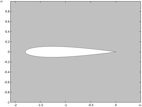
In the y text field, type c*0.594689181*(0.298222773*sqrt(s)-0.127125232*s-0.357907906*s^2+0.291984971*s^3-0.105174696*s^4).
|
|
5
|
|
1
|
|
2
|
Click in the Graphics window and then press Ctrl+A to select both objects.
|
|
1
|
|
2
|
|
3
|
|
4
|
On the object uni1, select Domain 2 only.
|
|
5
|
Click
|
|
6
|
Click
|
|
1
|
|
2
|
|
3
|
|
4
|
|
5
|
Click
|
|
6
|
|
1
|
|
2
|
|
3
|
Select the Keep input objects checkbox.
|
|
4
|
Click in the Graphics window and then press Ctrl+A to select both objects.
|
|
5
|
|
6
|
|
7
|
Click
|
|
8
|
|
1
|
|
2
|
|
3
|
|
1
|
|
2
|
Go to the Add Material window.
|
|
3
|
|
4
|
Click the Add to Component button in the window toolbar.
|
|
5
|
|
1
|
|
2
|
|
1
|
|
2
|
|
3
|
Click
|
|
4
|
|
5
|
Click OK.
|
|
6
|
|
7
|
|
1
|
|
2
|
|
3
|
Click
|
|
4
|
|
5
|
Click OK.
|
|
1
|
|
2
|
|
3
|
|
4
|
|
1
|
In the Model Builder window, under Component 1 (comp1) > Turbulent Flow, SST (spf) click Fluid Properties 1.
|
|
2
|
|
3
|
|
4
|
|
1
|
|
3
|
|
4
|
Click the Specify turbulence variables button.
|
|
5
|
|
6
|
|
7
|
|
8
|
|
1
|
|
2
|
|
3
|
Specify the u vector as
|
|
4
|
|
5
|
|
6
|
|
1
|
|
3
|
|
4
|
Click the Specify turbulence variables button.
|
|
5
|
|
6
|
|
1
|
|
2
|
|
3
|
|
5
|
Click to expand the Control Entities section. From the Smooth across removed control entities list, choose Off.
|
|
1
|
|
3
|
|
4
|
|
5
|
|
6
|
|
7
|
|
8
|
Select the Reverse direction checkbox.
|
|
1
|
|
3
|
|
4
|
|
5
|
|
6
|
|
7
|
|
1
|
|
3
|
|
4
|
|
5
|
|
6
|
|
7
|
|
8
|
Select the Reverse direction checkbox.
|
|
1
|
|
3
|
|
4
|
|
1
|
|
2
|
|
3
|
|
5
|
Locate the Control Entities section. From the Smooth across removed control entities list, choose Off.
|
|
1
|
|
3
|
|
4
|
|
5
|
|
6
|
|
7
|
|
1
|
|
3
|
|
4
|
|
5
|
|
6
|
|
7
|
|
8
|
Select the Symmetric distribution checkbox.
|
|
1
|
|
2
|
|
3
|
|
5
|
Locate the Control Entities section. From the Smooth across removed control entities list, choose Off.
|
|
1
|
|
3
|
|
4
|
|
5
|
|
6
|
|
7
|
|
1
|
|
3
|
|
4
|
|
5
|
|
6
|
|
7
|
|
8
|
Select the Reverse direction checkbox.
|
|
1
|
|
3
|
|
4
|
|
5
|
|
1
|
|
2
|
|
3
|
In the Solve for column of the table, under Component 1 (comp1), clear the checkbox for Turbulent Flow, SST (spf).
|
|
4
|
|
1
|
|
2
|
|
3
|
|
4
|
|
5
|
|
6
|
|
7
|
Click
|
|
1
|
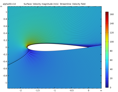
In the Model Builder window, right-click Velocity from Potential Flow Solution (ipf) and choose Streamline.
|
|
2
|
|
3
|
|
4
|
|
5
|
|
6
|
|
1
|
|
2
|
|
3
|
|
4
|
|
5
|
|
1
|
|
2
|
Go to the Add Study window.
|
|
3
|
Find the Studies subsection. In the Select Study tree, select Preset Studies for Selected Physics Interfaces > Turbulent Flow, SST > Stationary with Initialization.
|
|
4
|
Click the Add Study button in the window toolbar.
|
|
5
|
|
1
|
In the Settings window for Wall Distance Initialization, click to expand the Values of Dependent Variables section.
|
|
2
|
Find the Values of variables not solved for subsection. From the Settings list, choose User controlled.
|
|
3
|
|
4
|
|
1
|
|
2
|
|
3
|
In the Solve for column of the table, under Component 1 (comp1), clear the checkbox for Incompressible Potential Flow (ipf).
|
|
4
|
Click to expand the Values of Dependent Variables section. Find the Initial values of variables solved for subsection. From the Settings list, choose User controlled.
|
|
5
|
|
6
|
|
7
|
Click
|
|
9
|
|
1
|
|
3
|
|
5
|
|
6
|
Click
|
|
1
|
Go to the Table 1 window.
|
|
2
|
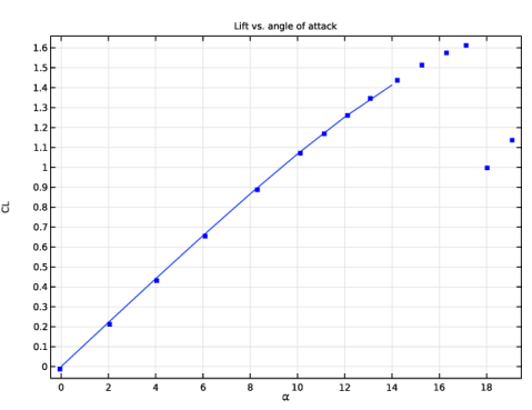
Click the Table Graph button in the window toolbar.
|
|
1
|
|
2
|
|
3
|
Click
|
|
4
|
Browse to the model’s Application Libraries folder and double-click the file naca0012_airfoil_Ladson_CL.dat.
|
|
1
|
|
2
|
|
3
|
|
4
|
Locate the Coloring and Style section. Find the Line style subsection. From the Line list, choose None.
|
|
5
|
|
6
|
|
1
|
|
2
|
|
3
|
|
4
|
|
5
|
Locate the Plot Settings section.
|
|
6
|
|
7
|
|
8
|
|
1
|
|
2
|
|
3
|
Click
|
|
4
|
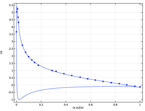
Browse to the model’s Application Libraries folder and double-click the file naca0012_airfoil_Gregory_OReilly_Cp.dat.
|
|
1
|
Go to the Table 3 window.
|
|
2
|
Click the Table Graph button in the window toolbar.
|
|
1
|
|
2
|
|
3
|
|
4
|
|
1
|
|
2
|
|
3
|
|
4
|
|
5
|
|
6
|
|
7
|
|
8
|
Click OK.
|
|
9
|
|
10
|
|
11
|
|
12
|
|
13
|
|
1
|
|
2
|
|
3
|
|
4
|
Locate the Plot Settings section.
|
|
5
|
|
6
|
|
7
|
|
1
|
|
2
|
|
3
|
|
1
|
|
2
|
|
3
|
|
4
|
|
5
|
Locate the Streamline Positioning section. From the Positioning list, choose Starting-point controlled.
|
|
6
|
|
7
|
|
8
|
|
9
|