
|
|
|
|
1
|
|
2
|
In the Select Physics tree, select Fluid Flow > Shallow Water Equations > Shallow Water Equations, Time Explicit (swe).
|
|
3
|
Click Add.
|
|
4
|
Click
|
|
5
|
|
6
|
Click
|
|
1
|
|
2
|
|
3
|
|
4
|
|
1
|
|
2
|
In the Settings window for Interpolation, type Inverse of Bottom Topography in the Label text field.
|
|
3
|
|
4
|
Click
|
|
5
|
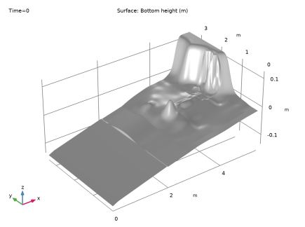
Browse to the model’s Application Libraries folder and double-click the file monai_runup_bathymetry.txt.
|
|
6
|
Click
|
|
7
|
Select the Use spatial coordinates as arguments checkbox.
|
|
8
|
Locate the Data Column Settings section. In the table, click to select the cell at row number 3 and column number 1.
|
|
9
|
|
10
|
|
1
|
|
2
|
|
3
|
|
4
|
Click
|
|
5
|
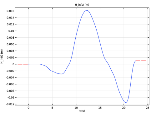
Browse to the model’s Application Libraries folder and double-click the file monai_runup_input_wave.txt.
|
|
6
|
Click
|
|
7
|
|
8
|
|
9
|
In the Function table, enter the following settings:
|
|
10
|
Click
|
|
1
|
|
2
|
|
3
|
|
4
|
|
5
|
|
1
|
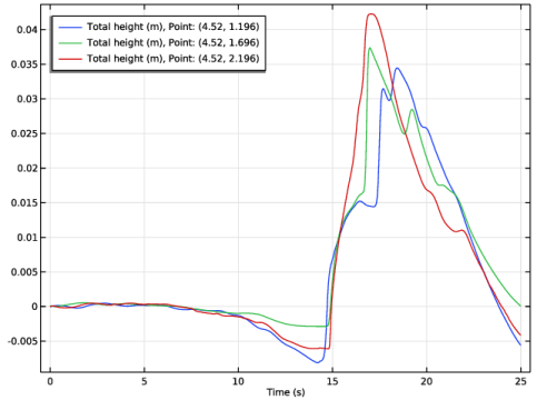
In the Model Builder window, expand the Probe (x,y)=(4.52,1.196) node, then click Point Probe Expression 1 (ppb1).
|
|
2
|
In the Settings window for Point Probe Expression, click Replace Expression in the upper-right corner of the Expression section. From the menu, choose Component 1 (comp1) > Shallow Water Equations, Time Explicit > swe.H - Total height - m.
|
|
1
|
|
2
|
In the Settings window for Domain Point Probe, type Probe (x,y)=(4.52,1.696) in the Label text field.
|
|
3
|
|
1
|
|
2
|
In the Settings window for Domain Point Probe, type Probe (x,y)=(4.52,2.196) in the Label text field.
|
|
3
|
|
1
|
In the Model Builder window, under Component 1 (comp1) > Shallow Water Equations, Time Explicit (swe) click Domain Properties 1.
|
|
2
|
|
3
|
|
1
|
|
2
|
|
3
|
|
1
|
|
3
|
|
4
|
|
5
|
|
6
|
|
1
|
|
2
|
|
3
|
Click the Custom button.
|
|
4
|
|
1
|
|
2
|
|
1
|
|
2
|
|
3
|
|
4
|
|
1
|
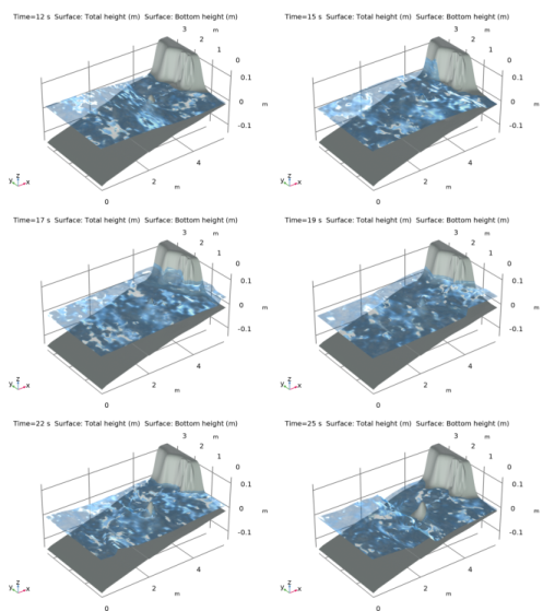
In the Model Builder window, expand the Results > Total Height (swe) > Total Height node, then click Height Expression 1.
|
|
2
|
|
3
|
|
4
|
Clear the Show height axis checkbox.
|
|
1
|
|
2
|
|
3
|
|
4
|
|
1
|
|
2
|
|
3
|
|
1
|
|
2
|
|
3
|