
|
|
|


|
1
|
|
2
|
In the Select Physics tree, select Fluid Flow > Single-Phase Flow > Large Eddy Simulation > LES RBVM (spf).
|
|
3
|
Click Add.
|
|
4
|
In the Select Physics tree, select Fluid Flow > Single-Phase Flow > Potential Flow > Incompressible Potential Flow (ipf).
|
|
5
|
Click Add.
|
|
6
|
Click
|
|
7
|
|
8
|
Click
|
|
1
|
|
2
|
|
1
|
|
2
|
|
3
|
|
4
|
Locate the Definition section. In the Expression text field, type -(besselj(0,3.1962)*besseli(0, 3.1962*x/(2*H))-besseli(0,3.1962)*besselj(0, 3.1962*x/(2*H)))*H/6.04844.
|
|
5
|
Locate the Plot Parameters section. In the table, enter the following settings:
|
|
1
|
|
2
|
|
3
|
|
4
|
|
5
|
|
6
|
|
7
|
|
1
|
|
2
|
|
3
|
|
4
|
Click
|
|
1
|
|
2
|
|
3
|
|
4
|
|
1
|
|
2
|
|
3
|
|
4
|
|
5
|
|
6
|
|
1
|
|
2
|
|
3
|
|
4
|
|
5
|
|
6
|
|
7
|
|
8
|
Locate the Selections of Resulting Entities section. Select the Resulting objects selection checkbox.
|
|
1
|
|
2
|
|
3
|
|
4
|
Click
|
|
1
|
|
2
|
|
3
|
|
4
|
|
5
|
|
1
|
|
2
|
|
3
|
|
4
|
|
5
|
|
1
|
|
2
|
|
3
|
|
4
|
|
5
|
|
1
|
|
2
|
|
3
|
|
4
|
|
5
|
Click OK.
|
|
1
|
|
2
|
|
3
|
|
4
|
|
5
|
Click OK.
|
|
6
|
|
7
|
|
8
|
|
9
|
Click OK.
|
|
1
|
|
2
|
|
3
|
|
4
|
|
5
|
Click OK.
|
|
6
|
|
1
|
|
2
|
|
3
|
|
1
|
|
2
|
|
3
|
|
4
|
|
1
|
In the Model Builder window, under Component 1 (comp1) > Incompressible Potential Flow (ipf) click Fluid Properties 1.
|
|
2
|
|
3
|
|
1
|
|
3
|
|
4
|
|
1
|
|
1
|
|
2
|
|
3
|
|
1
|
|
2
|
|
3
|
|
4
|
|
1
|
In the Model Builder window, under Component 1 (comp1) > LES RBVM (spf) right-click Initial Values 1 and choose Duplicate.
|
|
2
|
|
3
|
Specify the u vector as
|
|
4
|
|
1
|
|
2
|
|
3
|
|
1
|
|
3
|
|
4
|
|
5
|
Select the Include synthetic turbulence checkbox.
|
|
6
|
|
7
|
|
8
|
In the text field, type LTin.
|
|
9
|
|
1
|
|
3
|
|
4
|
Clear the Suppress backflow checkbox.
|
|
1
|
|
3
|
|
4
|
Click to select the
|
|
1
|
|
2
|
|
3
|
|
4
|
Click the Custom button.
|
|
5
|
|
6
|
|
1
|
|
1
|
|
3
|
|
4
|
|
1
|
|
3
|
|
4
|
|
5
|
|
6
|
|
7
|
|
8
|
Select the Reverse direction checkbox.
|
|
1
|
|
2
|
|
3
|
Click
|
|
5
|
|
1
|
|
1
|
|
2
|
|
3
|
|
4
|
|
5
|
|
6
|
|
7
|
Select the Symmetric distribution checkbox.
|
|
8
|
|
1
|
|
2
|
|
3
|
Clear the Generate default plots checkbox.
|
|
4
|
|
1
|
In the Model Builder window, under Study 1: Stationary Potential-Flow Solution click Step 1: Stationary.
|
|
2
|
|
3
|
In the Solve for column of the table, under Component 1 (comp1), clear the checkbox for LES RBVM (spf).
|
|
4
|
|
5
|
Select the Modify model configuration for study step checkbox.
|
|
6
|
|
7
|
Click
|
|
1
|
|
2
|
Go to the Add Study window.
|
|
3
|
Find the Physics interfaces in study subsection. In the table, clear the Solve checkbox for Incompressible Potential Flow (ipf).
|
|
4
|
|
5
|
Click the Add Study button in the window toolbar.
|
|
6
|
|
1
|
|
2
|
Clear the Generate default plots checkbox.
|
|
3
|
|
4
|
Locate the Study Settings section. Select the Store solution for all intermediate study steps checkbox.
|
|
1
|
In the Model Builder window, under Study 2: Time-Dependent LES Solution click Step 1: Time Dependent.
|
|
2
|
|
3
|
|
4
|
Click to expand the Values of Dependent Variables section. Find the Initial values of variables solved for subsection. From the Settings list, choose User controlled.
|
|
5
|
|
6
|
Find the Values of variables not solved for subsection. From the Settings list, choose User controlled.
|
|
7
|
|
8
|
|
1
|
|
2
|
|
3
|
|
4
|
|
5
|
|
6
|
Select the Clear source solution checkbox.
|
|
1
|
|
2
|
|
3
|
|
4
|
|
5
|
|
1
|
|
2
|
Go to the Add Study window.
|
|
3
|
|
4
|
Click the Add Study button in the window toolbar.
|
|
5
|
|
1
|
|
2
|
|
3
|
Clear the Generate default plots checkbox.
|
|
1
|
|
2
|
|
3
|
|
4
|
|
5
|
|
6
|
|
1
|
|
2
|
|
3
|
|
4
|
|
5
|
|
6
|
|
7
|
Select the Clear source solution checkbox.
|
|
8
|
|
9
|
|
1
|
|
2
|
|
3
|
|
4
|
Locate the Data section. From the Dataset list, choose Study 3: Time-Averaged LES Solution/Solution 4 (sol4).
|
|
5
|
|
1
|
|
2
|
|
3
|
Locate the Data section. From the Dataset list, choose Study 3: Time-Averaged LES Solution/Solution 4 (sol4).
|
|
4
|
|
5
|
|
6
|
Click OK.
|
|
1
|
|
2
|
|
3
|
Locate the Data section. From the Dataset list, choose Study 3: Time-Averaged LES Solution/Solution 4 (sol4).
|
|
4
|
|
1
|
|
2
|
|
3
|
Locate the Data section. From the Dataset list, choose Study 3: Time-Averaged LES Solution/Solution 4 (sol4).
|
|
4
|
|
1
|
|
2
|
|
3
|
|
4
|
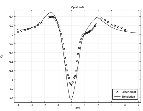
Browse to the model’s Application Libraries folder and double-click the file les_3d_hill_cp.txt.
|
|
5
|
|
6
|
|
7
|
Select the Only plot when requested checkbox.
|
|
1
|
|
2
|
|
3
|
Locate the Data section. From the Dataset list, choose Study 2: Time-Dependent LES Solution/Solution 2 (sol2).
|
|
4
|
|
5
|
|
6
|
Locate the Plot Settings section.
|
|
7
|
|
8
|
|
9
|
|
1
|
|
2
|
|
3
|
|
4
|
Locate the Coloring and Style section. Find the Line style subsection. From the Line list, choose None.
|
|
5
|
|
6
|
|
7
|
|
8
|
|
1
|
|
2
|
|
3
|
|
4
|
|
5
|
|
6
|
|
7
|
|
8
|
|
9
|
|
1
|
|
2
|
|
1
|
|
2
|
|
3
|
Locate the Data section. From the Dataset list, choose Study 3: Time-Averaged LES Solution/Solution 4 (sol4).
|
|
4
|
|
5
|
|
6
|
|
7
|
Select the Show trailing zeros checkbox.
|
|
8
|
|
1
|
|
2
|
|
3
|
|
4
|
|
5
|
|
6
|
In the Levels text field, type 3.08E-01 2.13E-01 1.19E-01 2.40E-02 -7.05E-02 -1.65E-01 -2.60E-01 -3.54E-01 -4.49E-01 -5.43E-01 -6.38E-01 -7.32E-01 -8.27E-01 -9.21E-01 -1.02E+00.
|
|
7
|
|
8
|
|
1
|
|
2
|
|
3
|
|
4
|
|
5
|
|
6
|
|
7
|
In the Levels text field, type 3.08E-01 2.13E-01 1.19E-01 2.40E-02 -7.05E-02 -1.65E-01 -2.60E-01 -3.54E-01 -4.49E-01 -5.43E-01 -6.38E-01 -7.32E-01 -8.27E-01 -9.21E-01 -1.02E+00.
|
|
8
|
|
9
|
|
10
|
Clear the Color legend checkbox.
|
|
1
|
|
2
|
|
1
|
|
2
|
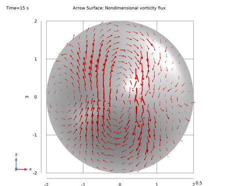
In the Settings window for 3D Plot Group, type Nondimensional Vorticity Flux in the Label text field.
|
|
3
|
Locate the Data section. From the Dataset list, choose Study 3: Time-Averaged LES Solution/Solution 4 (sol4).
|
|
4
|
|
5
|
|
6
|
Clear the Plot dataset edges checkbox.
|
|
7
|
|
8
|
Click
|
|
9
|
|
10
|
Click OK.
|
|
1
|
|
2
|
|
3
|
|
4
|
|
5
|
|
6
|
|
1
|
|
2
|
|
3
|
|
4
|
|
5
|
|
6
|
|
7
|
|
8
|
|
9
|
|
10
|
Locate the Coloring and Style section.
|
|
11
|
|
1
|
|
2
|
|
1
|
|
2
|
|
3
|
|
4
|
|
5
|
|
1
|
|
2
|
|
3
|
|
4
|
|
5
|
|
6
|
|
7
|
|
8
|
|
9
|
|
10
|
|
11
|
Locate the Coloring and Style section.
|
|
12
|
|
1
|
|
2
|
|
3
|
|
1
|
|
2
|
|
3
|
|
4
|
|
5
|
|
6
|
|
7
|
|
8
|
|
1
|
|
2
|
|
3
|
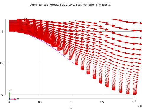
In the Logical expression for inclusion text field, type (u<=0) && (x>=0) && (x<=2*H) && (y<= 1.2*H).
|
|
1
|
|
2
|
|
1
|
|
2
|
|
3
|
|
4
|
|
5
|
|
1
|
|
2
|
|
3
|
|
4
|
|
5
|
|
6
|
|
7
|
|
8
|
|
9
|
|
10
|
|
11
|
Locate the Coloring and Style section.
|
|
12
|
|
1
|
|
2
|
|
3
|
|
1
|
|
2
|
|
1
|
|
2
|
|
3
|
Locate the Data section. From the Dataset list, choose Study 2: Time-Dependent LES Solution/Solution 2 (sol2).
|
|
4
|
|
5
|
|
6
|
|
1
|
|
2
|
|
3
|
|
4
|
|
5
|
|
6
|
|
1
|
|
2
|
|
3
|
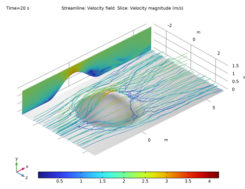
In the Logical expression for inclusion text field, type (x>=-4*H) && (x<=6*H) && (z>=-3*H) && (z<=3*H) && (y>=0) && (y<=1.5*H).
|
|
1
|
|
2
|
|
3
|
Clear the Plot dataset edges checkbox.
|
|
1
|
|
2
|
|
3
|
|
4
|
|
5
|
|
6
|
|
7
|
|
8
|
Locate the Coloring and Style section. Find the Line style subsection. From the Type list, choose Tube.
|
|
9
|
|
10
|
Select the Radius scale factor checkbox.
|
|
1
|
|
2
|
|
3
|
In the Logical expression for inclusion text field, type (x>=-4*H) && (x<=6*H) && (z>=-3*H) && (z<=3*H) && (y>=0) && (y<=1.5*H).
|
|
1
|
|
2
|
|
3
|
|
4
|
|
5
|
|
6
|
|
1
|
|
2
|
|
3
|
|
4
|
|
5
|
|
1
|
|
2
|
|
3
|
|
1
|
|
2
|
|
3
|
|
1
|
|
2
|
|
3
|
|
4
|
|
5
|
|
1
|
|
2
|
|
3
|
|
1
|
|
2
|
|
3
|
In the Logical expression for inclusion text field, type (x>=-4*H) && (x<=6*H) && (z>=-3*H) && (z<=3*H) && (y>=0) && (y<=1.5*H).
|
|
1
|
|
2
|
