PDF

Circulating Fluidized Bed
Introduction
This model simulates the operation of a circulating fluidized bed (CFB). In this apparatus, the dispersed phase, consisting of solid spherical particles, is fluidized by a gas and transported through a vertical riser. Upon reaching the outlet, the dispersed phase is reinjected in the vicinity of the gas inlet at the bottom of the bed. To study the flow in the fluidized bed, the model uses the Euler–Euler model. The phase properties and model setup follow those in Ref. 1.
Model Definition
Figure 1 displays the geometry of the fluidized bed and schematically describes its means of operation. The fluid phase, consisting of air, is injected at the bottom of the bed. The dispersed phase, particles with a diameter of 54 μm, are fluidized by the gas flow and transported upward. At the outlet, particles and gas exit the bed. The particles are fed back into the bed through reinjection inlets on the vertical walls near the gas inlet. The dispersed-phase flux matches that at the outlet, creating a circulating fluidized bed. Table 1 summarizes the bed geometries and the properties of the phases. The values correspond to those used in Ref. 1.
54 μm
1.8·10-5 kg/m3
Figure 1: Schematic of the circulating fluidized bed. The geometry is not to scale.
Governing Equations
Use the Euler–Euler model to solve for the flow of the continuous and dispersed phase. Both phases are then modeled as interpenetrating continua governed by a separate set of Navier-Stokes equations. The model also includes a transport equation for the dispersed-phase volume fraction. For details of the equations and assumptions used, see the theory section for the Euler–Euler Model, Laminar Flow interface in the CFD Module User’s Guide. To specify the transport properties of the fluidized bed, apply the settings below.
The viscosity of the dispersed phase is defined from the Gidaspow model as
where ϕd is the dispersed-phase volume fraction.
Assume the momentum transfer to be dominated by the drag force and the drag acting on each phase is given by a drag coefficient β in the manner of
Here, the subscripts “d” and “c” indicate properties of dispersed and continuous phase, respectively, and the slip velocity is defined as
To model the drag coefficient, use the Gidaspow drag model (Ref. 2)
for ϕc > 0.8 and
for ϕc < 0.8.
The dispersed phase transport resulting from particle–particle interaction, collisions, friction between particles, and so on, is included by the solids pressure term in the dispersed phase momentum equations. To model this term, the following expression is used (Ref. 1):
Initial Conditions
Initially all dispersed particles are positioned in a packed bed section at the bottom of the column. The packed bed section is 1.855 m high and consists of 50% particles. To avoid discontinuities at the start and end of the packed bed section, use a smoothly varying rectangle function to define the packed bed column.
Boundary Conditions
To fluidize the bed, air is injected at the bottom. Set the dispersed phase volume fraction at the inlet to zero.
Use pressure normal flow conditions for both phases at the outlet. To prevent the dispersed phase from falling back into the bed at the outflow boundary, remove the gravitational volume force in a region prior to the outlet using a smoothly varying step function.
At the vertical reinjection inlets, gas and solids are injected in a manner that matches the top outflux. This is achieved by using two coupling operators integrating the solid phase mass flux on the left and right sides of the bed center, each feeding the reinjection inlet on the respective side; see Figure 1. Apply solid mass flux which matches the mass outflux at the top. Use a gas velocity that equals that of the particles, assuming that the particle reinjection drags the gas phase along with it.
Along the solid bed walls, apply a no-slip condition for the continuous phase and a slip condition for the dispersed phase.
Results and Discussion
This section shows the results from the simulation. Note that the model is not deterministic and the plots may differ between computations performed on different platforms.
Figure 2 shows the startup phase of the fluidized bed simulation, plotting the dispersed-phase volume fraction during the first five seconds of simulation. Note that the packed bed section is pushed upward by the gas, primarily in the center of the bed. Due to the lower gas velocity close to the walls, the heavy solid phase is able to accumulate and fall down along the walls creating pockets with high concentration of solids. After about 6 s, the solid phase reaches the top of the bed and starts exiting the bed. You can verify this by inspecting the solids mass flux at the outlet; see Figure 3. This corresponds to the start of the re-injection of solids at the bottom. In the same figure, note that the bed reaches steady-state operations after about 15 s, after which the outflux of particles fluctuates around 11.5 kg/(m·s), which approximates to the experimental value reported in Ref. 1. Figure 4 shows snapshots of the dispersed-phase volume fraction during steady-state operation.
Figure 5 shows profiles of the averaged gas-phase streamwise velocity, giving an insight in the flow development. The gas-phase volume-fraction profiles at the corresponding positions are displayed in Figure 6.
Figure 2: Snapshots of the dispersed-phase volume fraction during the startup phase. Black indicates high volume fraction. The bed width has been scaled by a factor of ten.
Figure 3: Dispersed-phase bed outflux.
Figure 4: Snapshots of the dispersed-phase volume fraction during the steady-state operation. Black indicates high volume fraction. The bed width has been scaled by a factor of ten.
Figure 5: Averaged streamwise continuous-phase velocities at three vertical positions.
Figure 6: Averaged continuous-phase volume fractions at three vertical positions.
Notes About the COMSOL Implementation
The current model includes a slender geometry with an aspect ratio of about 100. When plotting and inspecting the solution over the whole modeling domain, it is therefore hard to distinguish any details. To produce the plots in Figure 2 and Figure 4, the view was stretched ten times in the x direction.
The flow in the fluidized bed is turbulent with Reynolds number around 9000. Nevertheless, a laminar flow model is used here. The effects of additional stresses from meso-scale structures are included in the models for solid pressure and inter-phase drag. See Ref. 4 for further details.
References
1. N. Yang, W. Wang, W. Ge, and J. Li, “CFD simulation of concurrent-up gas–solid flow in circulating fluidized beds with structure-dependent drag coefficient,” J. Chem. Eng., vol. 96, pp. 71–80, 2003.
2. D. Gidaspow, Multiphase Flow and Fluidization, Academic Press, San Diego, 1994.
3. H. Enwald, E. Peirano, and A.-E. Almstedt, “Eulerian Two-Phase Flow Theory Applied to Fluidization,” Int. J. Multiphase Flow, vol. 22, pp. 21–66, 1996.
4. K. Agrawal and others, “The Role of Meso-scale Structures in Rapid Gas-solid Flows,” J. Fluid Mech., vol. 445, pp. 151–185, 2001.
Application Library path: CFD_Module/Multiphase_Flow/fluidized_bed
Modeling Instructions
From the File menu, choose New.
New
In the New window, click  Model Wizard.
Model Wizard
1
In the Model Wizard window, click  2D.
2
In the Select Physics tree, select Fluid Flow > Multiphase Flow > Euler–Euler Model > Euler–Euler Model, Laminar Flow (ee).
3
Click Add.
4
Click  Study.
5
In the Select Study tree, select General Studies > Time Dependent.
6
Global Definitions
Parameters 1
1
In the Model Builder window, under Global Definitions click Parameters 1.
2
In the Settings window for Parameters, locate the Parameters section.
3
Click  Load from File.
4
Geometry 1
Rectangle 1 (r1)
1
In the Geometry toolbar, click  Rectangle.
2
In the Settings window for Rectangle, locate the Size and Shape section.
3
In the Width text field, type bedW.
4
In the Height text field, type bedH.
5
Locate the Position section. In the y text field, type inlH.
Rectangle 2 (r2)
1
In the Geometry toolbar, click  Rectangle.
2
In the Settings window for Rectangle, locate the Size and Shape section.
3
In the Width text field, type bedW.
4
In the Height text field, type solidH0.
5
Locate the Position section. In the y text field, type inlH.
Rectangle 3 (r3)
1
In the Geometry toolbar, click  Rectangle.
2
In the Settings window for Rectangle, locate the Size and Shape section.
3
In the Width text field, type bedW.
4
In the Height text field, type inlH.
Line Segment 1 (ls1)
1
In the Geometry toolbar, click  More Primitives and choose Line Segment.
2
In the Settings window for Line Segment, locate the Starting Point section.
3
From the Specify list, choose Coordinates.
4
Locate the Endpoint section. From the Specify list, choose Coordinates.
5
Locate the Starting Point section. In the y text field, type 0.02.
6
Locate the Endpoint section. In the y text field, type 0.02+injH.
Line Segment 2 (ls2)
1
Right-click Line Segment 1 (ls1) and choose Duplicate.
2
In the Settings window for Line Segment, locate the Starting Point section.
3
In the x text field, type bedW.
4
Locate the Endpoint section. In the x text field, type bedW.
Point 1 (pt1)
1
In the Geometry toolbar, click  Point.
2
In the Settings window for Point, locate the Point section.
3
In the x text field, type bedW/2.
4
In the y text field, type bedH+inlH.
5
In the Geometry toolbar, click  Build All.
Edit the view scale manually to rescale the geometry in the x direction and reduce the aspect ratio of plots.
Definitions
View 1
In the Model Builder window, expand the Component 1 (comp1) > Definitions node.
Axis
1
In the Model Builder window, expand the View 1 node, then click Axis.
2
In the Settings window for Axis, locate the Axis section.
3
From the View scale list, choose Manual.
4
In the x scale text field, type 10.
5
Click  Update.
6
Click the  Zoom Extents button in the Graphics toolbar.
View 2
1
In the Definitions toolbar, click  View.
2
In the Settings window for View, locate the View section.
3
Select the Lock axis checkbox.
Axis
1
In the Model Builder window, expand the View 2 node, then click Axis.
2
In the Settings window for Axis, locate the Axis section.
3
In the x minimum text field, type -0.01.
4
In the x maximum text field, type 0.105.
5
In the y maximum text field, type 0.4.
6
In the y minimum text field, type -0.025.
7
From the View scale list, choose Manual.
8
In the x scale text field, type 10.
9
Click  Update.
10
In the Graphics window toolbar, clicknext to  Go to Default View, then choose Go to View 1.
Create a step function to use for ramping up the bottom inlet velocity from zero to its full value over the initial 0.002 s.
Global Definitions
Step 1 (step1)
1
In the Home toolbar, click  Functions and choose Global > Step.
2
In the Settings window for Step, locate the Parameters section.
3
In the Location text field, type 1e-3[s].
4
Click to expand the Smoothing section. In the Size of transition zone text field, type 2e-3.
5
Click  Plot to view the step function.
Next, create another step function to use for ramping up the volume fraction at the reinjection slots.
Step 2 (step2)
1
In the Home toolbar, click  Functions and choose Global > Step.
2
In the Settings window for Step, locate the Parameters section.
3
In the Location text field, type bedH.
4
In the From text field, type 1.
5
In the To text field, type 0.
6
Locate the Smoothing section. In the Size of transition zone text field, type 0.15.
Create a rectangle function to specify the initial conditions for the solid volume fraction.
Rectangle 1 (rect1)
1
In the Home toolbar, click  Functions and choose Global > Rectangle.
2
In the Settings window for Rectangle, locate the Parameters section.
3
In the Lower limit text field, type inlH.
4
In the Upper limit text field, type solidH0+inlH.
5
Click to expand the Smoothing section. In the Size of transition zone text field, type bedW.
6
Create two integration operators at the outlet. You will use these to compute the dispersed phase outlet flux in the left and right bed halves as well as the corresponding reinjection velocities.
Definitions
Integration 1 (intop1)
1
In the Definitions toolbar, click  Nonlocal Couplings and choose Integration.
2
In the Settings window for Integration, type intopL in the Operator name text field.
3
Locate the Source Selection section. From the Geometric entity level list, choose Boundary.
4
Integration 2 (intop2)
1
In the Definitions toolbar, click  Nonlocal Couplings and choose Integration.
2
In the Settings window for Integration, type intopR in the Operator name text field.
3
Locate the Source Selection section. From the Geometric entity level list, choose Boundary.
4
Variables 1
1
In the Model Builder window, right-click Definitions and choose Variables.
2
In the Settings window for Variables, locate the Variables section.
3
Add a global probe for the dispersed phase outflux to get a plot automatically during the solver process.
Global Variable Probe: Dispersed phase outflux
1
In the Definitions toolbar, click  Probes and choose Global Variable Probe.
2
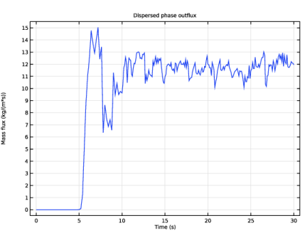
In the Settings window for Global Variable Probe, type Global Variable Probe: Dispersed phase outflux in the Label text field.
3
Locate the Expression section. In the Expression text field, type rhod*(outfluxdL+outfluxdR).
Euler–Euler Model, Laminar Flow (ee)
Phase Properties 1
1
In the Model Builder window, under Component 1 (comp1) > Euler–Euler Model, Laminar Flow (ee) click Phase Properties 1.
2
In the Settings window for Phase Properties, locate the Continuous Phase Properties section.
3
From the ρc list, choose User defined. In the associated text field, type rhoc.
4
From the μc list, choose User defined. In the associated text field, type muc.
5
Locate the Dispersed Phase Properties section. From the ρd list, choose User defined. In the associated text field, type rhod.
6
In the dd text field, type diam.
7
Locate the Viscosity Model section. From the μcm list, choose Pure phase value.
8
From the μdm list, choose Gidaspow.
9
Locate the Drag Model section. From the Drag model list, choose Gidaspow.
10
Locate the Solid Pressure Model section. From the Solid pressure model list, choose User-defined modulus of elasticity.
11
In the G text field, type 10^(6.385-8.686*ee.phicReg).
Initial Values 1
1
In the Model Builder window, click Initial Values 1.
2
In the Settings window for Initial Values, locate the Initial Values section.
3
In the phid text field, type phid0*rect1(y).
Wall 1
1
In the Model Builder window, click Wall 1.
2
In the Settings window for Wall, locate the Dispersed Phase Boundary Condition section.
3
From the Dispersed velocity boundary condition list, choose Slip.
4
Click the  Show More Options button in the Model Builder toolbar.
5
In the Show More Options dialog, click  Select All.
6
7
In the Model Builder window, click Euler–Euler Model, Laminar Flow (ee).
8
In the Settings window for Euler–Euler Model, Laminar Flow, click to expand the Consistent Stabilization section.
Use Limit small time steps effect on stabilization time scale instead of Use dynamic subgrid time scale to avoid loss of pressure stabilization at small time steps.
9
Clear the Use dynamic subgrid time scale checkbox.
10
Select the Limit small time steps effect on stabilization time scale checkbox.
Inlet 1
1
In the Physics toolbar, click  Boundaries and choose Inlet.
2
3
In the Settings window for Inlet, locate the Continuous Phase Boundary Condition section.
4
Specify the uc,0 vector as
5
Locate the Dispersed Phase Boundary Condition section. Specify the ud,0 vector as
6
From the Dispersed phase boundary condition list, choose No flux.
Outlet 1
1
In the Physics toolbar, click  Boundaries and choose Outlet.
2
3
In the Settings window for Outlet, locate the Mixture Boundary Condition section.
4
From the Mixture boundary condition list, choose Pressure normal flow.
Gravity 1
1
In the Physics toolbar, click  Domains and choose Gravity.
2
In the Settings window for Gravity, locate the Domain Selection section.
3
From the Selection list, choose All domains.
4
Locate the Acceleration of Gravity section. Specify the g vector as
Inlet 2
1
In the Physics toolbar, click  Boundaries and choose Inlet.
2
3
In the Settings window for Inlet, in the Graphics window toolbar, clicknext to  Go to Default View, then choose Go to View 2.
4
Locate the Two-Phase Inlet Type section. From the Two-phase inlet type list, choose Dispersed phase.
5
Locate the Continuous Phase Boundary Condition section. From the Continuous phase boundary condition list, choose Slip.
6
Locate the Dispersed Phase Boundary Condition section. Specify the ud,0 vector as
7
From the Dispersed phase boundary condition list, choose Mass flux.
8
In the text field, type max(intopL(ee.rhod*phid*udy),0)/injH.
Inlet 3
1
In the Physics toolbar, click  Boundaries and choose Inlet.
2
3
In the Settings window for Inlet, locate the Two-Phase Inlet Type section.
4
From the Two-phase inlet type list, choose Dispersed phase.
5
Locate the Continuous Phase Boundary Condition section. From the Continuous phase boundary condition list, choose Slip.
6
Locate the Dispersed Phase Boundary Condition section. Specify the ud,0 vector as
7
From the Dispersed phase boundary condition list, choose Mass flux.
8
In the text field, type max(intopR(ee.rhod*phid*udy),0)/injH.
Definitions
Maximum 1 (maxop1)
1
In the Definitions toolbar, click  Nonlocal Couplings and choose Maximum.
2
Click in the Graphics window and then press Ctrl+A to select all domains.
3
In the Settings window for Maximum, locate the Source Selection section.
4
From the Selection list, choose All domains.
5
Euler–Euler Model, Laminar Flow (ee)
Wall 2
1
In the Physics toolbar, click  Boundaries and choose Wall.
2
3
In the Settings window for Wall, locate the Continuous Phase Boundary Condition section.
4
From the Continuous velocity boundary condition list, choose Slip.
5
Locate the Dispersed Phase Boundary Condition section. From the Dispersed velocity boundary condition list, choose Slip.
6
In the Graphics window toolbar, clicknext to  Go to Default View, then choose Go to View 1.
Definitions
View 2
In the Model Builder window, under Component 1 (comp1) > Definitions right-click View 2 and choose Delete.
Mesh 1
Mapped 1
1
In the Mesh toolbar, click  Mapped.
2
In the Settings window for Mapped, locate the Domain Selection section.
3
From the Geometric entity level list, choose Entire geometry.
Distribution 1
1
Right-click Mapped 1 and choose Distribution.
2
3
In the Settings window for Distribution, locate the Distribution section.
4
In the Number of elements text field, type 40.
Distribution 2
1
In the Model Builder window, right-click Mapped 1 and choose Distribution.
2
3
In the Settings window for Distribution, locate the Distribution section.
4
In the Number of elements text field, type 53.
Distribution 3
1
Right-click Mapped 1 and choose Distribution.
2
3
In the Settings window for Distribution, locate the Distribution section.
4
In the Number of elements text field, type 300.
Distribution 4
1
Right-click Mapped 1 and choose Distribution.
2
3
In the Settings window for Distribution, locate the Distribution section.
4
From the Distribution type list, choose Predefined.
5
In the Number of elements text field, type 7.
6
In the Element ratio text field, type 3.
7
Select the Symmetric distribution checkbox.
Distribution 5
1
Right-click Mapped 1 and choose Distribution.
2
3
In the Settings window for Distribution, locate the Distribution section.
4
From the Distribution type list, choose Predefined.
5
In the Number of elements text field, type 6.
6
In the Element ratio text field, type 7.
Distribution 6
1
Right-click Mapped 1 and choose Distribution.
2
3
In the Settings window for Distribution, locate the Distribution section.
4
From the Distribution type list, choose Predefined.
5
In the Element ratio text field, type 3.
6
Select the Reverse direction checkbox.
7
Click  Build All.
Study 1
Step 1: Time Dependent
1
In the Model Builder window, under Study 1 click Step 1: Time Dependent.
2
In the Settings window for Time Dependent, locate the Study Settings section.
3
In the Output times text field, type range(0,0.2,10) range(10.1,0.1,30).
4
Right-click Study 1 > Step 1: Time Dependent and choose Get Initial Value for Step.
Results
Continuous Phase Velocity (ee)
1
In the Settings window for 2D Plot Group, locate the Plot Settings section.
2
Clear the Plot dataset edges checkbox.
Study 1
Step 1: Time Dependent
1
In the Model Builder window, under Study 1 click Step 1: Time Dependent.
2
In the Settings window for Time Dependent, click to expand the Results While Solving section.
3
Select the Plot checkbox  to monitor the velocity field throughout the computation.
Solver Configurations
In the Model Builder window, expand the Study 1 > Solver Configurations node.
Solution 1 (sol1)
1
In the Model Builder window, expand the Study 1 > Solver Configurations > Solution 1 (sol1) > Dependent Variables 1 node, then click Velocity Field, Continuous Phase (comp1.uc).
2
In the Settings window for Field, locate the Scaling section.
3
From the Method list, choose Manual.
4
In the Scale text field, type Uin.
5
In the Model Builder window, click Velocity Field, Dispersed Phase (comp1.ud).
6
In the Settings window for Field, locate the Scaling section.
7
From the Method list, choose Manual.
8
In the Scale text field, type Uin.
9
Results
Follow these instructions to reproduce the series of dispersed-phase volume fraction plots in Figure 2. Note the use of Deformation features to include a number of plots side-by-side in the same figure.
Continuous Phase Volume Fraction (ee)
1
In the Model Builder window, under Results click Continuous Phase Volume Fraction (ee).
2
In the Settings window for 2D Plot Group, locate the Plot Settings section.
3
Clear the Plot dataset edges checkbox.
4
Click to expand the Plot Array section. Select the Enable checkbox.
Surface 1
1
In the Model Builder window, expand the Continuous Phase Volume Fraction (ee) node, then click Surface 1.
2
In the Settings window for Surface, locate the Data section.
3
From the Dataset list, choose Study 1/Solution 1 (sol1).
4
From the Time (s) list, choose 0.
5
Click to expand the Title section. From the Title type list, choose None.
6
Click to expand the Range section. Locate the Coloring and Style section. Clear the Color legend checkbox.
Surface 2
1
Right-click Results > Continuous Phase Volume Fraction (ee) > Surface 1 and choose Duplicate.
2
In the Settings window for Surface, locate the Data section.
3
From the Time (s) list, choose 1.
4
Click to expand the Inherit Style section. From the Plot list, choose Surface 1.
Surface 3
1
Right-click Surface 2 and choose Duplicate.
2
In the Settings window for Surface, locate the Data section.
3
From the Time (s) list, choose 2.
Surface 4
1
Right-click Surface 3 and choose Duplicate.
2
In the Settings window for Surface, locate the Data section.
3
From the Time (s) list, choose 3.
Surface 5
1
Right-click Surface 4 and choose Duplicate.
2
In the Settings window for Surface, locate the Data section.
3
From the Time (s) list, choose 4.
Surface 6
1
Right-click Surface 5 and choose Duplicate.
2
In the Settings window for Surface, locate the Data section.
3
From the Time (s) list, choose 5.
4
In the Continuous Phase Volume Fraction (ee) toolbar, click  Plot.
5
Click the  Zoom Extents button in the Graphics toolbar.
Use the plot group you just created as the starting point for reproducing Figure 4.
Dispersed Phase Volume Fraction at Steady-State
1
In the Model Builder window, right-click Continuous Phase Volume Fraction (ee) and choose Duplicate.
2
In the Settings window for 2D Plot Group, type Dispersed Phase Volume Fraction at Steady-State in the Label text field.
3
In the Dispersed Phase Volume Fraction at Steady-State toolbar, click  Plot.
Surface 1
1
In the Model Builder window, expand the Dispersed Phase Volume Fraction at Steady-State node, then click Surface 1.
2
In the Settings window for Surface, locate the Data section.
3
From the Time (s) list, choose 20.
Surface 2
1
In the Model Builder window, click Surface 2.
2
In the Settings window for Surface, locate the Data section.
3
From the Time (s) list, choose 22.
Surface 3
1
In the Model Builder window, click Surface 3.
2
In the Settings window for Surface, locate the Data section.
3
From the Time (s) list, choose 24.
Surface 4
1
In the Model Builder window, click Surface 4.
2
In the Settings window for Surface, locate the Data section.
3
From the Time (s) list, choose 26.
Surface 5
1
In the Model Builder window, click Surface 5.
2
In the Settings window for Surface, locate the Data section.
3
From the Time (s) list, choose 28.
Surface 6
1
In the Model Builder window, click Surface 6.
2
In the Settings window for Surface, locate the Data section.
3
From the Time (s) list, choose 30.
4
In the Dispersed Phase Volume Fraction at Steady-State toolbar, click  Plot.
5
Click the  Zoom Extents button in the Graphics toolbar.
The following steps reproduce the plot shown in Figure 3.
Dispersed Phase Bed Outflux
1
In the Results toolbar, click  1D Plot Group.
2
In the Settings window for 1D Plot Group, type Dispersed Phase Bed Outflux in the Label text field.
3
Click to expand the Title section. From the Title type list, choose Manual.
4
In the Title text area, type Dispersed phase outflux.
5
Locate the Plot Settings section.
6
Select the y-axis label checkbox. In the associated text field, type Mass flux (kg/(m*s)).
Global 1
1
Right-click Dispersed Phase Bed Outflux and choose Global.
2
In the Settings window for Global, locate the y-Axis Data section.
3
4
Click to expand the Legends section. Clear the Show legends checkbox.
5
In the Dispersed Phase Bed Outflux toolbar, click  Plot.
To reproduce the plots in Figure 6 and Figure 5, begin by creating three cut line datasets.
Cut Line 2D 1
1
In the Results toolbar, click  Cut Line 2D.
2
In the Settings window for Cut Line 2D, locate the Line Data section.
3
In row Point 1, set y to 1.
4
In row Point 2, set y to 1 and x to bedW.
5
Clear the Bounded by points checkbox.
Cut Line 2D 2
1
Right-click Cut Line 2D 1 and choose Duplicate.
2
In the Settings window for Cut Line 2D, locate the Line Data section.
3
In row Point 1, set y to 3.5.
4
In row Point 2, set y to 3.5.
Cut Line 2D 3
1
Right-click Cut Line 2D 2 and choose Duplicate.
2
In the Settings window for Cut Line 2D, locate the Line Data section.
3
In row Point 1, set y to 8.75.
4
In row Point 2, set y to 8.75.
Now plot the time-averaged continuous phase volume fraction at the three y positions defined by the cut line datasets you just defined. Compare the resulting plot with that in Figure 6.
1D Plot Group 6
In the Results toolbar, click  1D Plot Group.
Line Graph 1
1
Right-click 1D Plot Group 6 and choose Line Graph.
2
In the Settings window for Line Graph, locate the Data section.
3
From the Dataset list, choose Cut Line 2D 1.
4
From the Time selection list, choose First.
5
Locate the y-Axis Data section. In the Expression text field, type 1-timeavg(10,30,phid).
6
Locate the x-Axis Data section. From the Parameter list, choose Expression.
7
In the Expression text field, type Xg/bedW.
8
Click to expand the Legends section. Select the Show legends checkbox.
9
From the Legends list, choose Manual.
10
Line Graph 2
1
Right-click Line Graph 1 and choose Duplicate.
2
In the Settings window for Line Graph, locate the Data section.
3
From the Dataset list, choose Cut Line 2D 2.
4
Locate the Legends section. In the table, enter the following settings:
Line Graph 3
1
Right-click Line Graph 2 and choose Duplicate.
2
In the Settings window for Line Graph, locate the Data section.
3
From the Dataset list, choose Cut Line 2D 3.
4
Locate the Legends section. In the table, enter the following settings:
Averaged Continuous Phase Volume Fraction
1
In the Model Builder window, under Results click 1D Plot Group 6.
2
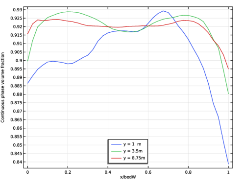
In the Settings window for 1D Plot Group, type Averaged Continuous Phase Volume Fraction in the Label text field.
3
Locate the Title section. From the Title type list, choose None.
4
Locate the Plot Settings section.
5
Select the x-axis label checkbox. In the associated text field, type x/bedW.
6
Select the y-axis label checkbox. In the associated text field, type Continuous phase volume fraction.
7
Locate the Legend section. From the Position list, choose Lower middle.
8
In the Averaged Continuous Phase Volume Fraction toolbar, click  Plot.
Finally, reproduce Figure 5 by duplicating and adapting the plot group you just created.
Averaged Continuous Phase Velocity
1
Right-click Averaged Continuous Phase Volume Fraction and choose Duplicate.
2
In the Model Builder window, click Averaged Continuous Phase Volume Fraction 1.
3
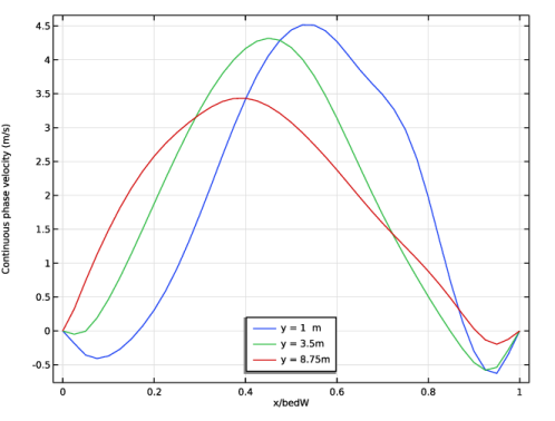
In the Settings window for 1D Plot Group, type Averaged Continuous Phase Velocity in the Label text field.
4
Locate the Plot Settings section. In the y-axis label text field, type Continuous phase velocity (m/s).
Line Graph 1
1
In the Model Builder window, click Line Graph 1.
2
In the Settings window for Line Graph, locate the y-Axis Data section.
3
In the Expression text field, type timeavg(10,30,ucy).
Line Graph 2
1
In the Model Builder window, click Line Graph 2.
2
In the Settings window for Line Graph, locate the y-Axis Data section.
3
In the Expression text field, type timeavg(10,30,ucy).
Line Graph 3
1
In the Model Builder window, click Line Graph 3.
2
In the Settings window for Line Graph, locate the y-Axis Data section.
3
In the Expression text field, type timeavg(10,30,ucy).
4
In the Averaged Continuous Phase Velocity toolbar, click  Plot.