PDF

FDA Benchmark Blood Pump
Introduction
Centrifugal pumps are widely used in medical applications. Fluid-structure interaction is a vital aspect of a variety of medical devices. A centrifugal blood pump is one such device that uses a rotating impeller to pump blood.
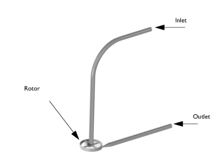
Figure 1: Geometry of the centrifugal blood pump.
This model features a centrifugal blood pump with four filleted blades (3 mm tall and 3 mm wide) placed at 90° angle on a 4 mm thick rotor base; see Figure 1. The CAD geometry used in this model is taken from Ref. 1.
Disclaimer: CFD and blood damage validation studies were performed at the Food and Drug Administration (FDA) by employees of the Federal Government in the course of their official duties. Pursuant to Title 17, Section 105 of the United States Code, the CAD file obtained from the FDA is not subject to copyright protection and is in the public domain. Permission is hereby granted, free of charge, to any person obtaining a copy of the study results, to deal in such CAD file without restriction, including without limitation the rights to use, copy, modify, merge, publish, distribute, sublicense, or sell copies of such CAD file or derivatives, and to permit persons to whom such CAD file is furnished to do so. FDA assumes no responsibility whatsoever for use by other parties of the such CAD file, its contents or documentation, and makes no guarantees, expressed or implied, about its quality, reliability, or any other characteristic. Further, use of this CAD file in no way implies endorsement by the FDA or confers any advantage in regulatory decisions. Although this CAD file can be redistributed and/or modified freely, we ask that any derivative works bear some notice that they are derived from it, and any modified versions bear some notice that they have been modified.
Model Definition
Following the FDA guidelines, the blood is assumed to be a Newtonian fluid. The k-ε turbulence model is used to obtain an initial flow solution for the shear stress transport (SST) model, which is subsequently used to obtain flow solutions with higher accuracy. Inlet flow rates of 2.5–7 L/min at a pump speed of 3500 rpm are simulated. A frozen rotor approach is used to compute the (pseudo) steady-state solution.
Results and Discussion
Table 1 shows a summary of wall shear stress and torque values. The maximum wall shear stress magnitude is computed over the housing rim (the 180° segment nearest the outlet) and also wall maximum shear stress magnitude is computed over the fillet around cutwater. The shaft torque value is computed from the integral of the total stress.
In Ref. 2, FDA published its benchmark centrifugal blood pump study, reporting results from computational studies as well as the data from its experiments. The experimental data is extracted from the graphs in the publication and compared with the results of the centrifugal benchmark blood pump model in order to validate the CFD results.
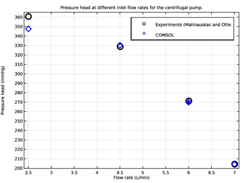
The pressure head across the pump is computed at a pump speed of 3500 rpm for several flow rates. The computed results show good agreement with the experimental results from Ref. 2, as is shown in Figure 2.
Figure 2: Pressure head at different inlet flow rates for the centrifugal pump operating at 3500 rpm.
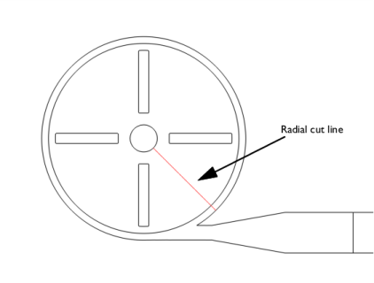
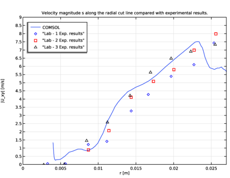
The velocity magnitude at pump condition of 6 L/min and 3500 rpm is computed at the upper blade plane. The velocity magnitude, inside the blood pump model, based on the x- and y-velocity components along the radial cut line (see Figure 3) match the measurements qualitatively and are consistent with what is reported in other CFD studies Ref. 2. The results of the comparison are presented in Figure 4.
Figure 3: Radial cut line at upper blade plane.
Figure 4: The velocity magnitude based on the x- and y-velocity components along the radial cut line compared with experimental data Ref. 2.
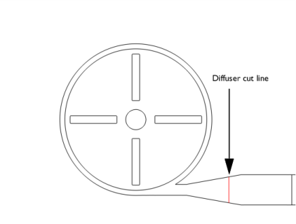
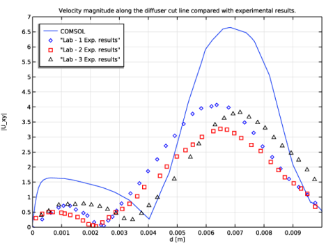
Similarly, the velocity profile was computed at x = 0.035 m in the diffuser region Figure 5 at a pump condition of 6 L/min and 3500 rpm. Figure 6 shows that the computed velocity magnitudes match the measurements qualitatively and are consistent with what is reported in Ref. 2.
Figure 5: Diffuser cut line.
Figure 6: Velocity magnitude inside the blood pump based on the x- and y-velocity components along the diffuser cut line compared with experimental results from Ref. 2.
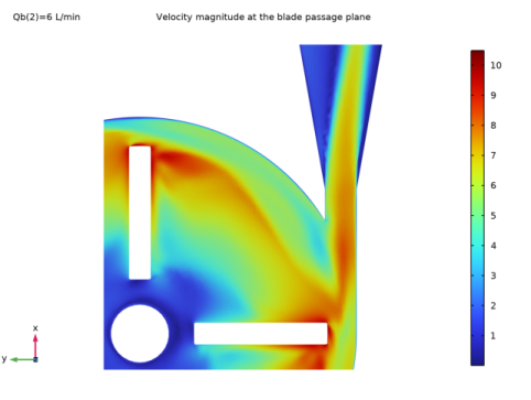
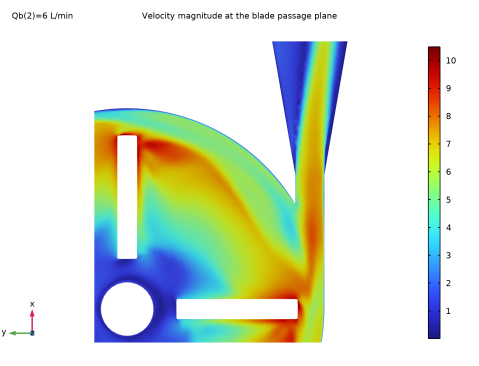
The interpolated contours of the three-dimensional velocity magnitude for the upper-blade passage plane under operating condition of 3500 rpm and an inlet flow rate of 6 L/min are plotted in Figure 7. The results qualitatively match those in Ref. 2.
Figure 7: Velocity magnitude at the blade passage plane under operating condition of 3500 rpm and an inlet flow rate of 6 L/min.
References
1. Computational Fluid Dynamics Round Robin Study: github.com/OSEL-DAM/CFD-and-Blood-Damage-Benchmarks/tree/main.
2. R.A. Malinauskas and others, “FDA benchmark medical device flow models for CFD validation,” ASAIO Journal, vol. 63, no. 2, pp. 150–160, 2017.
Application Library path: CFD_Module/Verification_Examples/fda_benchmark_blood_pump
Modeling Instructions
From the File menu, choose New.
New
In the New window, click  Model Wizard.
Model Wizard
1
In the Model Wizard window, click  3D.
2
In the Select Physics tree, select Fluid Flow > Single-Phase Flow > Turbulent Flow > Turbulent Flow, k-ε (spf).
3
Click Add.
4
Click  Study.
5
In the Select Study tree, select Empty Study.
6
Global Definitions
Parameters 1
1
In the Model Builder window, under Global Definitions click Parameters 1.
2
In the Settings window for Parameters, locate the Parameters section.
3
Geometry 1
Create the geometry. To simplify this step, insert a prepared geometry sequence.
1
In the Model Builder window, under Component 1 (comp1) click Geometry 1.
2
In the Settings window for Geometry, locate the Advanced section.
3
From the Geometry representation list, choose CAD kernel.
4
In the Geometry toolbar, click Insert Sequence and choose Insert Sequence.
5
Full geometry instructions can be found at the end of the document.
6
In the Geometry toolbar, click  Build All.
Disable the analysis of the geometry as the remaining small geometric details are needed.
7
In the Model Builder window, click Geometry 1.
8
Locate the Cleanup section. Clear the Automatic detection of small details checkbox.
Materials
Blood
1
In the Model Builder window, under Component 1 (comp1) right-click Materials and choose Blank Material.
2
In the Settings window for Material, type Blood in the Label text field.
3
Locate the Material Contents section. In the table, enter the following settings:
Component 1 (comp1)
A Moving Mesh is used to rotate the impeller/rotor.
Rotating Domain 1
1
In the Physics toolbar, click  Moving Mesh and choose Rotating Domain.
2
In the Settings window for Rotating Domain, locate the Domain Selection section.
3
Click  Clear Selection.
4
Click  Paste Selection.
5
In the Paste Selection dialog, type 2 in the Selection text field.
6
7
In the Settings window for Rotating Domain, locate the Rotation section.
8
From the Rotation type list, choose Specified rotational velocity.
9
From the Rotational velocity expression list, choose Constant revolutions per time.
10
In the f text field, type rp.
The turbulent flow in the pump is resolved using a RANS model. To obtain initial values for the SST model, a k-ε model is first solved in Study 1.
Turbulent Flow, k-ε - Prelim
1
In the Model Builder window, under Component 1 (comp1) click Turbulent Flow, k-ε (spf).
2
In the Settings window for Turbulent Flow, k-ε, type Turbulent Flow, k-[epsilon ]- Prelim in the Label text field.
Wall 2
1
In the Model Builder window, expand the Component 1 (comp1) > Turbulent Flow, k-ε - Prelim (spf) node.
2
Right-click Component 1 (comp1) > Turbulent Flow, k-ε - Prelim (spf) and choose Wall.
3
In the Settings window for Wall, click to expand the Wall Movement section.
4
From the Translational velocity list, choose Zero (Fixed wall).
5
Locate the Boundary Selection section. Click  Paste Selection.
6
In the Paste Selection dialog, type 7 in the Selection text field.
7
Inlet 1
1
In the Physics toolbar, click  Boundaries and choose Inlet.
2
In the Settings window for Inlet, locate the Boundary Selection section.
3
Click  Paste Selection.
4
In the Paste Selection dialog, type 54 in the Selection text field.
5
6
In the Settings window for Inlet, locate the Boundary Condition section.
7
From the list, choose Fully developed flow.
8
Locate the Fully Developed Flow section. Click the Flow rate button.
9
In the V0 text field, type Qb.
Outlet 1
1
In the Physics toolbar, click  Boundaries and choose Outlet.
2
In the Settings window for Outlet, locate the Boundary Selection section.
3
Click  Paste Selection.
4
In the Paste Selection dialog, type 55 in the Selection text field.
5
Mesh 1
1
In the Model Builder window, under Component 1 (comp1) click Mesh 1.
2
In the Settings window for Mesh, locate the Physics-Controlled Mesh section.
3
In the table, clear the Use checkbox for Geometric Analysis, Detail Size.
4
Locate the Sequence Type section. From the list, choose User-controlled mesh.
Size
1
In the Model Builder window, under Component 1 (comp1) > Mesh 1 click Size.
2
In the Settings window for Size, click to expand the Element Size Parameters section.
3
Locate the Element Size section. From the Predefined list, choose Fine.
4
Locate the Element Size Parameters section. In the Minimum element size text field, type 1e-3.
Size 1
In the Model Builder window, right-click Size 1 and choose Delete. Click Yes to confirm.
Corner Refinement 1
Right-click Corner Refinement 1 and choose Delete. Click Yes to confirm.
Free Triangular 1
1
In the Mesh toolbar, click  More Generators and choose Free Triangular.
2
3
Right-click Free Triangular 1 and choose Move Up.
4
Right-click Free Triangular 1 and choose Move Up.
Size 1
1
Right-click Free Triangular 1 and choose Size.
2
In the Settings window for Size, locate the Element Size section.
3
From the Calibrate for list, choose Fluid dynamics.
4
From the Predefined list, choose Finer.
5
Click the Custom button.
6
Locate the Element Size Parameters section.
7
Select the Maximum element size checkbox. In the associated text field, type 1e-4.
8
Select the Minimum element size checkbox. In the associated text field, type 1e-7.
Free Tetrahedral 1
1
In the Model Builder window, under Component 1 (comp1) > Mesh 1 click Free Tetrahedral 1.
2
In the Settings window for Free Tetrahedral, locate the Domain Selection section.
3
From the Geometric entity level list, choose Domain.
4
Click  Paste Selection.
5
In the Paste Selection dialog, type 1 2 in the Selection text field.
6
Size 1
1
In the Model Builder window, right-click Free Tetrahedral 1 and choose Size.
2
In the Settings window for Size, locate the Geometric Entity Selection section.
3
Click  Clear Selection.
4
Click  Paste Selection.
5
In the Paste Selection dialog, type 2 in the Selection text field.
6
7
In the Settings window for Size, locate the Element Size section.
8
From the Calibrate for list, choose Fluid dynamics.
9
Click the Custom button.
10
Locate the Element Size Parameters section.
11
Select the Maximum element size checkbox. In the associated text field, type 1e-3.
12
Select the Minimum element size checkbox. In the associated text field, type 4e-4.
Size 2
1
In the Model Builder window, right-click Free Tetrahedral 1 and choose Size.
2
In the Settings window for Size, locate the Geometric Entity Selection section.
3
Click  Clear Selection.
4
Click  Paste Selection.
5
In the Paste Selection dialog, type 1 in the Selection text field.
6
7
In the Settings window for Size, locate the Element Size section.
8
From the Calibrate for list, choose Fluid dynamics.
9
Click the Custom button.
10
Locate the Element Size Parameters section.
11
Select the Maximum element size checkbox. In the associated text field, type 1e-3.
12
Select the Minimum element size checkbox. In the associated text field, type 1e-7.
13
Select the Maximum element growth rate checkbox. In the associated text field, type 1.4.
14
Select the Curvature factor checkbox.
15
Select the Resolution of narrow regions checkbox.
Free Tetrahedral 1
In the Model Builder window, right-click Free Tetrahedral 1 and choose Size.
Size 3
1
In the Settings window for Size, locate the Geometric Entity Selection section.
2
From the Geometric entity level list, choose Boundary.
3
Click  Paste Selection.
4
In the Paste Selection dialog, type 9-13, 28-33 in the Selection text field.
5
6
In the Settings window for Size, locate the Element Size section.
7
From the Calibrate for list, choose Fluid dynamics.
8
From the Predefined list, choose Finer.
9
Click the Custom button.
10
Locate the Element Size Parameters section.
11
Select the Maximum element size checkbox. In the associated text field, type 1e-3.
12
Select the Minimum element size checkbox. In the associated text field, type 4e-4.
13
Click  Build Selected.
Swept 1
1
In the Mesh toolbar, click  Swept.
2
Drag and drop below Free Tetrahedral 1.
3
In the Settings window for Swept, locate the Domain Selection section.
4
From the Geometric entity level list, choose Domain.
5
Click  Paste Selection.
6
In the Paste Selection dialog, type 3 4 5 6 in the Selection text field.
7
Distribution 1
1
In the Model Builder window, right-click Swept 1 and choose Distribution.
2
In the Settings window for Distribution, locate the Domain Selection section.
3
Click  Clear Selection.
4
Click  Paste Selection.
5
In the Paste Selection dialog, type 3 in the Selection text field.
6
7
In the Settings window for Distribution, locate the Distribution section.
8
From the Distribution type list, choose Predefined.
9
In the Number of elements text field, type 60.
10
In the Element ratio text field, type 3.
11
Select the Symmetric distribution checkbox.
Distribution 2
1
In the Model Builder window, right-click Swept 1 and choose Distribution.
2
In the Settings window for Distribution, locate the Domain Selection section.
3
Click  Clear Selection.
4
Click  Paste Selection.
5
In the Paste Selection dialog, type 4 in the Selection text field.
6
7
In the Settings window for Distribution, locate the Distribution section.
8
From the Distribution type list, choose Predefined.
9
In the Number of elements text field, type 70.
10
In the Element ratio text field, type 1.
Distribution 3
1
Right-click Swept 1 and choose Distribution.
2
In the Settings window for Distribution, locate the Domain Selection section.
3
Click  Clear Selection.
4
Click  Paste Selection.
5
In the Paste Selection dialog, type 5 in the Selection text field.
6
7
In the Settings window for Distribution, locate the Distribution section.
8
From the Distribution type list, choose Predefined.
9
In the Number of elements text field, type 100.
10
In the Element ratio text field, type 2.
Distribution 4
1
Right-click Swept 1 and choose Distribution.
2
In the Settings window for Distribution, locate the Domain Selection section.
3
Click  Clear Selection.
4
Click  Paste Selection.
5
In the Paste Selection dialog, type 6 in the Selection text field.
6
7
In the Settings window for Distribution, locate the Distribution section.
8
From the Distribution type list, choose Predefined.
9
In the Number of elements text field, type 30.
10
In the Element ratio text field, type 2.
Boundary Layers 1
1
In the Model Builder window, under Component 1 (comp1) > Mesh 1 click Boundary Layers 1.
2
In the Settings window for Boundary Layers, locate the Geometric Entity Selection section.
3
4
From the Geometric entity level list, choose Entire geometry.
5
Click to expand the Corner Settings section. From the Handling of sharp edges list, choose Splitting.
Boundary Layer Properties 1
1
In the Model Builder window, expand the Boundary Layers 1 node, then click Boundary Layer Properties 1.
2
In the Settings window for Boundary Layer Properties, locate the Layers section.
3
In the Number of layers text field, type 8.
4
In the Thickness adjustment factor text field, type 1.1.
5
Click  Build All.
Study 1
Step 1: Frozen Rotor
1
In the Study toolbar, click  More Study Steps and choose Stationary > Frozen Rotor.
A Frozen Rotor study is used to compute the steady-state flow involving the rotating machinery.
2
In the Model Builder window, click Study 1.
3
In the Settings window for Study, locate the Study Settings section.
4
Clear the Generate default plots checkbox.
5
In the Label text field, type Study 1 - k-epsilon.
Solution 1 (sol1)
1
In the Study toolbar, click  Show Default Solver.
2
Click  Compute.
Definitions
Wall Boundaries
1
In the Model Builder window, expand the Component 1 (comp1) > Definitions node.
2
Right-click Definitions and choose Selections > Explicit.
3
In the Settings window for Explicit, type Wall Boundaries in the Label text field.
4
Locate the Input Entities section. From the Geometric entity level list, choose Boundary.
5
Click  Paste Selection.
6
In the Paste Selection dialog, type 1-4, 7, 9-19, 22, 23, 28-33, 40-51 in the Selection text field.
7
Inlet Pressure
1
In the Definitions toolbar, click  Probes and choose Boundary Probe.
2
In the Settings window for Boundary Probe, locate the Source Selection section.
3
From the Selection list, choose Manual.
4
Click  Clear Selection.
5
Click  Paste Selection.
6
In the Paste Selection dialog, type 54 in the Selection text field.
7
8
In the Settings window for Boundary Probe, type Inlet Pressure in the Label text field.
9
In the Variable name text field, type p_in.
10
Locate the Expression section. In the Expression text field, type spf2.pA.
11
In the Table and plot unit field, type Pa.
Outlet Pressure
1
In the Definitions toolbar, click  Probes and choose Boundary Probe.
2
In the Settings window for Boundary Probe, type Outlet Pressure in the Label text field.
3
In the Variable name text field, type p_out.
4
Locate the Source Selection section. Click  Clear Selection.
5
Click  Paste Selection.
6
In the Paste Selection dialog, type 55 in the Selection text field.
7
8
In the Settings window for Boundary Probe, locate the Expression section.
9
In the Expression text field, type spf2.pA.
10
In the Table and plot unit field, type Pa.
11
Click to expand the Table and Window Settings section. Click  Add Plot Window.
An important indicator of less trauma to red blood cells and a lower systemic inflammatory response is shear stress.
Maximum Wall Shear Stress - Housing Rim
1
In the Definitions toolbar, click  Probes and choose Boundary Probe.
2
In the Settings window for Boundary Probe, type Maximum Wall Shear Stress - Housing Rim in the Label text field.
3
In the Variable name text field, type tau_housing_max.
4
Locate the Probe Type section. From the Type list, choose Maximum.
5
Locate the Source Selection section. Click  Clear Selection.
6
Click  Copy Selection.
7
Click  Paste Selection.
8
In the Paste Selection dialog, type 1 in the Selection text field.
9
10
In the Settings window for Boundary Probe, locate the Expression section.
11
In the Expression text field, type spf2.u_tauWall^2*spf2.rho.
12
In the Table and plot unit field, type N/m^2.
13
Click to expand the Table and Window Settings section. Click  Add Plot Window.
Maximum Wall Shear Stress - Fillet
1
In the Definitions toolbar, click  Probes and choose Boundary Probe.
2
In the Settings window for Boundary Probe, type Maximum Wall Shear Stress - Fillet in the Label text field.
3
In the Variable name text field, type tau_fillet_max.
4
Locate the Probe Type section. From the Type list, choose Maximum.
5
Locate the Source Selection section. From the Selection list, choose Manual.
6
Click  Clear Selection.
7
8
Locate the Expression section. In the Expression text field, type spf2.u_tauWall^2*spf2.rho.
9
Click to expand the Table and Window Settings section. Click  Add Plot Window.
Shaft Torque
1
In the Definitions toolbar, click  Probes and choose Boundary Probe.
2
In the Settings window for Boundary Probe, type Shaft Torque in the Label text field.
3
In the Variable name text field, type shaft_torque.
4
Locate the Probe Type section. From the Type list, choose Integral.
5
Locate the Source Selection section. Click  Clear Selection.
6
Click  Paste Selection.
7
In the Paste Selection dialog, type 28-31 in the Selection text field.
8
9
In the Settings window for Boundary Probe, locate the Expression section.
10
In the Expression text field, type x*spf2.T_tracy-y*spf2.T_tracx.
11
In the Table and plot unit field, type nN*m.
12
Locate the Table and Window Settings section. Click  Add Plot Window.
Average 1 (aveop1)
1
In the Definitions toolbar, click  Nonlocal Couplings and choose Average.
2
In the Settings window for Average, locate the Source Selection section.
3
From the Geometric entity level list, choose Boundary.
4
Click  Paste Selection.
5
In the Paste Selection dialog, type 21 in the Selection text field.
6
Average 2 (aveop2)
1
In the Definitions toolbar, click  Nonlocal Couplings and choose Average.
2
In the Settings window for Average, locate the Source Selection section.
3
From the Geometric entity level list, choose Boundary.
4
Click  Paste Selection.
5
In the Paste Selection dialog, type 55 in the Selection text field.
6
Turbulent Flow, k-ε - Prelim (spf)
Generate New Turbulence Model Interface 1
1
In the Physics toolbar, click  Global and choose Generate New Turbulence Model Interface.
2
In the Settings window for Generate New Turbulence Model Interface, locate the Study section.
3
From the Initial value from study list, choose Study 1 - k-epsilon.
4
Locate the Turbulence Model Interface section. From the list, choose Turbulent Flow, SST.
5
Locate the Model Generation section. Click Create.
Turbulent Flow, SST 2 (spf2)
Wall 1
1
In the Model Builder window, expand the Turbulent Flow, SST 2 (spf2) node, then click Wall 1.
2
In the Settings window for Wall, click to expand the Wall Movement section.
3
From the Translational velocity list, choose Automatic from frame.
Study 2 - SST
1
In the Model Builder window, click Study 2.
2
In the Settings window for Study, type Study 2 - SST in the Label text field.
3
Locate the Study Settings section. Clear the Generate default plots checkbox.
4
In the Home toolbar, click  Compute.
The Generate New Turbulence Model option is used to create a turbulent flow interface using the SST model solved with Study 2. This also generates initial values for the new interface based on the solution from Study 1.
Add Study
1
In the Home toolbar, click  Add Study to open the Add Study window.
2
Go to the Add Study window.
3
Find the Studies subsection. In the Select Study tree, select Empty Study.
4
Click the Add Study button in the window toolbar.
5
In the Home toolbar, click  Add Study to close the Add Study window.
Study 3
Step 1: Frozen Rotor
1
In the Study toolbar, click  More Study Steps and choose Stationary > Frozen Rotor.
2
In the Settings window for Frozen Rotor, locate the Physics and Variables Selection section.
3
In the Solve for column of the table, under Component 1 (comp1), clear the checkbox for Turbulent Flow, k-ε - Prelim (spf).
4
In the Model Builder window, click Study 3.
5
In the Settings window for Study, type Study 3 - SST - Qb Sweep in the Label text field.
6
In the Model Builder window, click Step 1: Frozen Rotor.
7
In the Settings window for Frozen Rotor, click to expand the Values of Dependent Variables section.
8
Find the Initial values of variables solved for subsection. From the Settings list, choose User controlled.
9
From the Method list, choose Solution.
10
From the Study list, choose Study 2 - SST, Frozen Rotor.
11
Find the Values of variables not solved for subsection. From the Settings list, choose User controlled.
12
From the Study list, choose Study 2 - SST, Frozen Rotor.
13
From the Method list, choose Solution.
14
Click to expand the Study Extensions section. Select the Auxiliary sweep checkbox.
15
16
Solution 4 (sol4)
1
In the Study toolbar, click  Show Default Solver.
2
Click  Compute.
Results
Exterior Walls, Study 3 - SST - Qb Sweep/Solution 4
1
In the Model Builder window, expand the Results > Datasets node.
2
Right-click Results > Datasets and choose Surface.
3
In the Settings window for Surface, type Exterior Walls, Study 3 - SST - Qb Sweep/Solution 4 in the Label text field.
4
Locate the Data section. From the Dataset list, choose Study 3 - SST - Qb Sweep/Solution 4 (sol4).
5
Locate the Selection section. From the Selection list, choose Wall Boundaries.
Exterior Walls, Study 2 - SST/Solution 2
1
Right-click Exterior Walls, Study 3 - SST - Qb Sweep/Solution 4 and choose Duplicate.
2
In the Settings window for Surface, type Exterior Walls, Study 2 - SST/Solution 2 in the Label text field.
3
Locate the Data section. From the Dataset list, choose Study 2 - SST/Solution 2 (sol2).
4
Locate the Selection section. From the Selection list, choose Wall Boundaries.
Blade Passage Plane
1
In the Results toolbar, click  Cut Plane.
2
In the Settings window for Cut Plane, type Blade Passage Plane in the Label text field.
3
Locate the Data section. From the Dataset list, choose Study 2 - SST/Solution 2 (sol2).
4
Locate the Plane Data section. From the Plane list, choose xy-planes.
5
In the z-coordinate text field, type 0.006562.
Lower Gap Plane
1
In the Results toolbar, click  Cut Plane.
2
In the Settings window for Cut Plane, type Lower Gap Plane in the Label text field.
3
Locate the Data section. From the Dataset list, choose Study 2 - SST/Solution 2 (sol2).
4
Locate the Plane Data section. From the Plane list, choose xy-planes.
5
In the z-coordinate text field, type 0.0005.
zx Outlet Plane
1
In the Results toolbar, click  Cut Plane.
2
In the Settings window for Cut Plane, type zx Outlet Plane in the Label text field.
3
Locate the Data section. From the Dataset list, choose Study 2 - SST/Solution 2 (sol2).
4
Locate the Plane Data section. From the Plane list, choose zx-planes.
5
In the y-coordinate text field, type -0.027805.
Upper Gap Plane
1
In the Results toolbar, click  Cut Plane.
2
In the Settings window for Cut Plane, type Upper Gap Plane in the Label text field.
3
Locate the Data section. From the Dataset list, choose Study 2 - SST/Solution 2 (sol2).
4
Locate the Plane Data section. From the Plane list, choose xy-planes.
5
In the z-coordinate text field, type 0.0085.
zx Inlet Plane
1
In the Results toolbar, click  Cut Plane.
2
In the Settings window for Cut Plane, type zx Inlet Plane in the Label text field.
3
Locate the Data section. From the Dataset list, choose Study 2 - SST/Solution 2 (sol2).
4
Locate the Plane Data section. From the Plane list, choose zx-planes.
yz Inlet Plane
1
In the Results toolbar, click  Cut Plane.
2
In the Settings window for Cut Plane, type yz Inlet Plane in the Label text field.
3
Locate the Data section. From the Dataset list, choose Study 2 - SST/Solution 2 (sol2).
Upper Blade Plane
1
In the Results toolbar, click  Cut Plane.
2
In the Settings window for Cut Plane, type Upper Blade Plane in the Label text field.
3
Locate the Data section. From the Dataset list, choose Study 2 - SST/Solution 2 (sol2).
4
Locate the Plane Data section. From the Plane list, choose xy-planes.
5
In the z-coordinate text field, type 8[mm]-1.2[mm].
Radial Cut Line 2D
1
In the Results toolbar, click  Cut Line 2D.
2
In the Settings window for Cut Line 2D, type Radial Cut Line 2D in the Label text field.
3
Locate the Data section. From the Dataset list, choose Upper Blade Plane.
4
Locate the Line Data section. In row Point 2, set x to 0.03*cos(45[deg]).
5
In row Point 2, set y to -0.03*cos(45[deg]).
Diffuser Cut Line 2D
1
In the Results toolbar, click  Cut Line 2D.
2
In the Settings window for Cut Line 2D, type Diffuser Cut Line 2D in the Label text field.
3
Locate the Data section. From the Dataset list, choose Upper Blade Plane.
4
Locate the Line Data section. In row Point 1, set x to 0.0367.
5
In row Point 2, set x to 0.0367.
6
In row Point 2, set y to -0.04.
Imported Experimental Results - Radial Cut Line 1
1
In the Results toolbar, click  Table.
2
In the Settings window for Table, type Imported Experimental Results - Radial Cut Line 1 in the Label text field.
3
Locate the Data section. Click  Import.
4
5
Locate the Column Headers section. In the table, enter the following settings:
Imported Experimental Results - Radial Cut Line 2
1
In the Results toolbar, click  Table.
2
In the Settings window for Table, type Imported Experimental Results - Radial Cut Line 2 in the Label text field.
3
Locate the Data section. Click  Import.
4
5
Locate the Column Headers section. In the table, enter the following settings:
Imported Experimental Results - Radial Cut Line 3
1
In the Results toolbar, click  Table.
2
In the Settings window for Table, type Imported Experimental Results - Radial Cut Line 3 in the Label text field.
3
Locate the Data section. Click  Import.
4
5
Locate the Column Headers section. In the table, enter the following settings:
Imported Experimental Results -Diffuser Cut Line 1
1
In the Results toolbar, click  Table.
2
In the Settings window for Table, type Imported Experimental Results -Diffuser Cut Line 1 in the Label text field.
3
Locate the Data section. Click  Import.
4
5
Locate the Column Headers section. In the table, enter the following settings:
Imported Experimental Results -Diffuser Cut Line 2
1
In the Results toolbar, click  Table.
2
In the Settings window for Table, type Imported Experimental Results -Diffuser Cut Line 2 in the Label text field.
3
Locate the Data section. Click  Import.
4
5
Locate the Column Headers section. In the table, enter the following settings:
Imported Experimental Results -Diffuser Cut Line 3
1
In the Results toolbar, click  Table.
2
In the Settings window for Table, type Imported Experimental Results -Diffuser Cut Line 3 in the Label text field.
3
Locate the Data section. Click  Import.
4
5
Locate the Column Headers section. In the table, enter the following settings:
Imported - Experimental Results - Pressure Head
1
In the Results toolbar, click  Table.
2
In the Settings window for Table, type Imported - Experimental Results - Pressure Head in the Label text field.
3
Locate the Data section. Click  Import.
4
5
Locate the Column Headers section. In the table, enter the following settings:
Pressure Head - Study 3
1
In the Results toolbar, click  Global Evaluation.
2
In the Settings window for Global Evaluation, type Pressure Head - Study 3 in the Label text field.
3
Locate the Data section. From the Dataset list, choose Study 3 - SST - Qb Sweep/Solution 4 (sol4).
4
Locate the Expressions section. In the table, enter the following settings:
5
Clicknext to  Evaluate, then choose New Table.
Pressure Head - Study 3
1
In the Model Builder window, under Results > Tables click Table 9.
2
In the Settings window for Table, type Pressure Head - Study 3 in the Label text field.
Pressure Head - Study 2
1
In the Results toolbar, click  Global Evaluation.
2
In the Settings window for Global Evaluation, type Pressure Head - Study 2 in the Label text field.
3
Locate the Data section. From the Dataset list, choose Study 2 - SST/Solution 2 (sol2).
4
Locate the Expressions section. In the table, enter the following settings:
5
Clicknext to  Evaluate, then choose New Table.
Pressure Head - Study 2
1
In the Model Builder window, under Results > Tables click Table 10.
2
In the Settings window for Table, type Pressure Head - Study 2 in the Label text field.
Surface Integration 1 - Inflow
1
In the Results toolbar, click  More Derived Values and choose Integration > Surface Integration.
2
In the Settings window for Surface Integration, type Surface Integration 1 - Inflow in the Label text field.
3
4
Locate the Data section. From the Dataset list, choose Study 2 - SST/Solution 2 (sol2).
5
Locate the Expressions section. In the table, enter the following settings:
Surface Integration 1 - Outflow
1
In the Results toolbar, click  More Derived Values and choose Integration > Surface Integration.
2
In the Settings window for Surface Integration, type Surface Integration 1 - Outflow in the Label text field.
3
4
Locate the Data section. From the Dataset list, choose Study 2 - SST/Solution 2 (sol2).
5
Locate the Expressions section. In the table, enter the following settings:
Probe Plot Group 1
1
In the Model Builder window, under Results click Probe Plot Group 1.
2
In the Settings window for 1D Plot Group, locate the Legend section.
3
Clear the Show legends checkbox.
4
Locate the Plot Settings section.
5
Select the y-axis label checkbox. In the associated text field, type Absolute pressure (Pa).
6
Click to expand the Title section. From the Title type list, choose Manual.
7
In the Title text area, type Inlet Pressure.
Probe Plot Group 2
1
In the Model Builder window, click Probe Plot Group 2.
2
In the Settings window for 1D Plot Group, locate the Legend section.
3
Clear the Show legends checkbox.
4
Locate the Plot Settings section.
5
Select the y-axis label checkbox. In the associated text field, type Absolute pressure (Pa).
6
Click to expand the Title section. From the Title type list, choose Manual.
7
In the Title text area, type Outlet Pressure.
Probe Plot Group 3
1
In the Model Builder window, expand the Probe Plot Group 2 node, then click Results > Probe Plot Group 3.
2
In the Settings window for 1D Plot Group, locate the Legend section.
3
Clear the Show legends checkbox.
4
Locate the Plot Settings section.
5
Select the y-axis label checkbox. In the associated text field, type Maximum Wall Shear Stress (N/m^2).
6
Click to expand the Title section. From the Title type list, choose Manual.
7
In the Title text area, type Maximum Wall Shear Stress on Housing Rim.
Probe Plot Group 4
1
In the Model Builder window, click Probe Plot Group 4.
2
In the Settings window for 1D Plot Group, locate the Legend section.
3
Clear the Show legends checkbox.
4
Locate the Plot Settings section.
5
Select the y-axis label checkbox. In the associated text field, type Maximum Wall Shear Stress.
6
Click to expand the Title section. From the Title type list, choose Manual.
7
In the Title text area, type Maximum Wall Shear Stress on Fillet.
8
In the Probe Plot Group 4 toolbar, click  Plot.
Probe Plot Group 5
1
In the Model Builder window, click Probe Plot Group 5.
2
In the Settings window for 1D Plot Group, locate the Legend section.
3
Clear the Show legends checkbox.
4
Locate the Plot Settings section.
5
Select the y-axis label checkbox. In the associated text field, type Shaft Torque (nN*m).
Definitions
View 8
1
In the Model Builder window, under Component 1 (comp1) right-click Definitions and choose View.
2
In the Settings window for View, locate the View section.
3
Select the Show axis units checkbox.
4
Clear the Show grid checkbox.
Hide for Geometry 1
1
Right-click View 8 and choose Hide for Geometry.
2
In the Settings window for Hide for Geometry, locate the Selection section.
3
From the Geometric entity level list, choose Boundary.
4
Click the  Paste Selection button for Selection.
5
In the Paste Selection dialog, type 4-6, 8, 14, 16, 18, 20-22, 24-27, 34-37, 39, 42, 45, 47, 48, 50-52, 54, 55 in the Selection text field.
6
Results
Velocity (spf2)
1
In the Model Builder window, under Results click Velocity (spf2).
2
In the Settings window for 3D Plot Group, click to expand the Title section.
3
From the Title type list, choose None.
4
Locate the Plot Settings section. Clear the Plot dataset edges checkbox.
5
From the View list, choose View 8.
6
Locate the Data section. From the Dataset list, choose Study 2 - SST/Solution 2 (sol2).
Surface 1
1
Right-click Velocity (spf2) and choose Surface.
2
In the Settings window for Surface, locate the Coloring and Style section.
3
Clear the Color legend checkbox.
4
Locate the Data section. From the Dataset list, choose Blade Passage Plane.
5
Locate the Expression section. In the Expression text field, type spf2.U.
Transparency 1
Right-click Surface 1 and choose Transparency.
Surface 2
1
In the Model Builder window, right-click Velocity (spf2) and choose Surface.
2
In the Settings window for Surface, locate the Data section.
3
From the Dataset list, choose zx Outlet Plane.
4
Locate the Expression section. In the Expression text field, type spf2.U.
5
Locate the Coloring and Style section. Clear the Color legend checkbox.
Transparency 1
Right-click Surface 2 and choose Transparency.
Surface 3
1
In the Model Builder window, right-click Velocity (spf2) and choose Surface.
2
In the Settings window for Surface, locate the Data section.
3
From the Dataset list, choose zx Inlet Plane.
4
Locate the Expression section. In the Expression text field, type spf2.U.
5
Locate the Coloring and Style section. Clear the Color legend checkbox.
Transparency 1
Right-click Surface 3 and choose Transparency.
Velocity (spf2)
Right-click Surface 3 > Transparency 1 and choose Surface.
Surface 4
1
In the Settings window for Surface, locate the Data section.
2
From the Dataset list, choose Study 2 - SST/Solution 2 (sol2).
3
Locate the Coloring and Style section. From the Coloring list, choose Uniform.
4
From the Color list, choose Gray.
5
In the Velocity (spf2) toolbar, click  Plot.
Pressure (spf2)
1
In the Model Builder window, under Results click Pressure (spf2).
2
In the Settings window for 3D Plot Group, locate the Data section.
3
From the Dataset list, choose Exterior Walls, Study 2 - SST/Solution 2.
Surface
1
In the Model Builder window, expand the Pressure (spf2) node, then click Surface.
2
In the Settings window for Surface, locate the Data section.
3
From the Dataset list, choose Blade Passage Plane.
4
Locate the Expression section. In the Expression text field, type p2.
Pressure (spf2)
Right-click Surface and choose Surface.
Surface 2
1
In the Settings window for Surface, locate the Data section.
2
From the Dataset list, choose zx Outlet Plane.
3
Locate the Expression section. In the Expression text field, type p2.
4
Locate the Coloring and Style section. Clear the Color legend checkbox.
5
In the Pressure (spf2) toolbar, click  Plot.
Wall Resolution (spf2)
1
In the Model Builder window, under Results click Wall Resolution (spf2).
2
In the Settings window for 3D Plot Group, locate the Data section.
3
From the Dataset list, choose Study 2 - SST/Solution 2 (sol2).
Turbulent Viscosity
1
In the Results toolbar, click  3D Plot Group.
2
In the Settings window for 3D Plot Group, type Turbulent Viscosity in the Label text field.
3
Locate the Data section. From the Dataset list, choose Study 2 - SST/Solution 2 (sol2).
Surface 1
1
Right-click Turbulent Viscosity and choose Surface.
2
In the Settings window for Surface, locate the Data section.
3
From the Dataset list, choose Blade Passage Plane.
4
Locate the Expression section. In the Expression text field, type spf2.muT.
Surface 2
1
In the Model Builder window, right-click Turbulent Viscosity and choose Surface.
2
In the Settings window for Surface, locate the Data section.
3
From the Dataset list, choose zx Outlet Plane.
4
Locate the Expression section. In the Expression text field, type spf2.muT.
5
Locate the Coloring and Style section. Clear the Color legend checkbox.
Turbulent Viscosity
1
In the Model Builder window, click Turbulent Viscosity.
2
In the Turbulent Viscosity toolbar, click  Plot.
Magnitude of Uxy - Radial
1
In the Results toolbar, click  1D Plot Group.
2
In the Settings window for 1D Plot Group, locate the Plot Settings section.
3
Select the x-axis label checkbox.
4
Select the y-axis label checkbox.
5
In the x-axis label text field, type r [m].
6
In the y-axis label text field, type |U_xy| [m/s].
7
Click to expand the Title section. From the Title type list, choose Manual.
8
In the Title text area, type Velocity magnitude s along the radial cut line compared with experimental results..
9
In the Label text field, type Magnitude of Uxy - Radial.
10
Locate the Data section. From the Dataset list, choose Radial Cut Line 2D.
11
Locate the Plot Settings section. Select the x-axis label checkbox.
12
Select the y-axis label checkbox.
13
In the x-axis label text field, type r [m].
14
In the y-axis label text field, type |U_xy| [m/s].
15
Click to expand the Title section. From the Title type list, choose Manual.
16
In the Title text area, type Velocity magnitude s along the radial cut line compared with experimental results..
17
Locate the Axis section. Select the Manual axis limits checkbox.
18
In the x minimum text field, type 0.
19
In the x maximum text field, type 0.027.
20
In the y minimum text field, type 0.
21
In the y maximum text field, type 9.
22
Locate the Legend section. From the Position list, choose Upper left.
Line Graph 1
1
Right-click Magnitude of Uxy - Radial and choose Line Graph.
2
In the Settings window for Line Graph, locate the y-Axis Data section.
3
In the Expression text field, type sqrt(u2^2+v2^2).
4
Locate the x-Axis Data section. From the Parameter list, choose Expression.
5
In the Expression text field, type sqrt(x^2+y^2).
6
Click to expand the Legends section. Select the Show legends checkbox.
7
From the Legends list, choose Manual.
8
9
In the Magnitude of Uxy - Radial toolbar, click  Plot.
Table Graph 1
1
In the Model Builder window, right-click Magnitude of Uxy - Radial and choose Table Graph.
2
In the Settings window for Table Graph, locate the Data section.
3
From the Table list, choose Imported Experimental Results - Radial Cut Line 1.
4
From the x-axis data list, choose r [m].
5
Locate the Coloring and Style section. Find the Line style subsection. From the Line list, choose None.
6
From the Color list, choose Blue.
7
Find the Line markers subsection. From the Marker list, choose Diamond.
8
From the Positioning list, choose In data points.
9
Click to expand the Legends section. Select the Show legends checkbox.
10
From the Legends list, choose Manual.
11
12
In the Magnitude of Uxy - Radial toolbar, click  Plot.
Table Graph 2
1
Right-click Magnitude of Uxy - Radial and choose Table Graph.
2
In the Settings window for Table Graph, locate the Data section.
3
From the Table list, choose Imported Experimental Results - Radial Cut Line 2.
4
From the x-axis data list, choose r [m].
5
Locate the Coloring and Style section. Find the Line style subsection. From the Line list, choose None.
6
From the Color list, choose Red.
7
Find the Line markers subsection. From the Marker list, choose Square.
8
From the Positioning list, choose In data points.
9
Click to expand the Legends section. Select the Show legends checkbox.
10
From the Legends list, choose Manual.
11
12
In the Magnitude of Uxy - Radial toolbar, click  Plot.
Table Graph 3
1
Right-click Magnitude of Uxy - Radial and choose Table Graph.
2
In the Settings window for Table Graph, locate the Data section.
3
From the Table list, choose Imported Experimental Results - Radial Cut Line 3.
4
From the x-axis data list, choose r [m].
5
Locate the Coloring and Style section. Find the Line style subsection. From the Line list, choose None.
6
From the Color list, choose Black.
7
Find the Line markers subsection. From the Marker list, choose Triangle.
8
From the Positioning list, choose In data points.
9
Click to expand the Legends section. Select the Show legends checkbox.
10
From the Legends list, choose Manual.
11
12
In the Magnitude of Uxy - Radial toolbar, click  Plot.
Magnitude of Uxy - Diffuser
1
In the Results toolbar, click  1D Plot Group.
2
In the Settings window for 1D Plot Group, type Magnitude of Uxy - Diffuser in the Label text field.
3
Locate the Data section. From the Dataset list, choose Diffuser Cut Line 2D.
4
Locate the Plot Settings section. Select the x-axis label checkbox.
5
Select the y-axis label checkbox.
6
In the x-axis label text field, type d [m].
7
In the y-axis label text field, type |U_xy|.
8
Locate the Title section. From the Title type list, choose Manual.
9
In the Title text area, type Velocity magnitude along the diffuser cut line compared with experimental results..
10
Locate the Axis section. Select the Manual axis limits checkbox.
11
In the x minimum text field, type 0.
12
In the x maximum text field, type 0.01.
13
In the y minimum text field, type 0.
14
In the y maximum text field, type 7.
15
Locate the Legend section. From the Position list, choose Upper left.
Line Graph 1
1
Right-click Magnitude of Uxy - Diffuser and choose Line Graph.
2
In the Settings window for Line Graph, locate the y-Axis Data section.
3
In the Expression text field, type sqrt(u2^2+v2^2).
4
Click to expand the Legends section. Select the Show legends checkbox.
5
From the Legends list, choose Manual.
6
7
In the Magnitude of Uxy - Diffuser toolbar, click  Plot.
Table Graph 1
1
In the Model Builder window, right-click Magnitude of Uxy - Diffuser and choose Table Graph.
2
In the Settings window for Table Graph, locate the Data section.
3
From the Table list, choose Imported Experimental Results -Diffuser Cut Line 1.
4
From the x-axis data list, choose d [m].
5
Locate the Coloring and Style section. Find the Line style subsection. From the Line list, choose None.
6
From the Color list, choose Blue.
7
Find the Line markers subsection. From the Marker list, choose Diamond.
8
From the Positioning list, choose In data points.
9
Click to expand the Legends section. Select the Show legends checkbox.
10
From the Legends list, choose Manual.
11
12
In the Magnitude of Uxy - Diffuser toolbar, click  Plot.
Table Graph 2
1
Right-click Magnitude of Uxy - Diffuser and choose Table Graph.
2
In the Settings window for Table Graph, locate the Data section.
3
From the Table list, choose Imported Experimental Results -Diffuser Cut Line 2.
4
From the x-axis data list, choose d [m].
5
Locate the Coloring and Style section. Find the Line style subsection. From the Line list, choose None.
6
From the Color list, choose Red.
7
Find the Line markers subsection. From the Marker list, choose Square.
8
From the Positioning list, choose In data points.
9
Click to expand the Legends section. Select the Show legends checkbox.
10
From the Legends list, choose Manual.
11
12
In the Magnitude of Uxy - Diffuser toolbar, click  Plot.
Table Graph 3
1
Right-click Magnitude of Uxy - Diffuser and choose Table Graph.
2
In the Settings window for Table Graph, locate the Data section.
3
From the Table list, choose Imported Experimental Results -Diffuser Cut Line 3.
4
From the x-axis data list, choose d [m].
5
Locate the Coloring and Style section. Find the Line style subsection. From the Line list, choose None.
6
From the Color list, choose Black.
7
Find the Line markers subsection. From the Marker list, choose Triangle.
8
From the Positioning list, choose In data points.
9
Click to expand the Legends section. Select the Show legends checkbox.
10
From the Legends list, choose Manual.
11
12
In the Magnitude of Uxy - Diffuser toolbar, click  Plot.
Pressure Head - Exp. Comparison
1
In the Results toolbar, click  1D Plot Group.
2
In the Settings window for 1D Plot Group, type Pressure Head - Exp. Comparison in the Label text field.
3
Locate the Title section. From the Title type list, choose Manual.
4
In the Title text area, type Pressure head at different inlet flow rates for the centrifugal pump..
5
Locate the Plot Settings section.
6
Select the x-axis label checkbox. In the associated text field, type Flow rate (L/min).
7
Select the y-axis label checkbox. In the associated text field, type Pressure head (mmHg).
Table Graph 1
1
Right-click Pressure Head - Exp. Comparison and choose Table Graph.
2
In the Settings window for Table Graph, locate the Data section.
3
From the Table list, choose Imported - Experimental Results - Pressure Head.
4
From the x-axis data list, choose Flow rate(L/min).
5
Locate the Coloring and Style section. Find the Line style subsection. From the Line list, choose None.
6
From the Color list, choose Black.
7
From the Width list, choose 6.
8
Find the Line markers subsection. From the Marker list, choose Circle.
9
Locate the Legends section. From the Legends list, choose Manual.
10
Select the Show legends checkbox.
11
Table Graph 2
1
In the Model Builder window, right-click Pressure Head - Exp. Comparison and choose Table Graph.
2
In the Settings window for Table Graph, locate the Data section.
3
From the Table list, choose Pressure Head - Study 3.
4
Locate the Coloring and Style section. Find the Line style subsection. From the Line list, choose None.
5
From the Color list, choose Blue.
6
From the Width list, choose 6.
7
Find the Line markers subsection. From the Marker list, choose Diamond.
8
Locate the Legends section. Select the Show legends checkbox.
9
From the Legends list, choose Manual.
10
Table Graph 3
1
Right-click Pressure Head - Exp. Comparison and choose Table Graph.
2
In the Settings window for Table Graph, locate the Data section.
3
From the Table list, choose Pressure Head - Study 2.
4
From the x-axis data list, choose Inlet flow rate (L/min).
5
Locate the Coloring and Style section. Find the Line style subsection. From the Line list, choose Solid.
6
From the Color list, choose Blue.
7
From the Width list, choose 6.
8
Find the Line markers subsection. From the Marker list, choose Diamond.
9
In the Pressure Head - Exp. Comparison toolbar, click  Plot.
Velocity magnitude at the blade passage plane
1
In the Results toolbar, click  3D Plot Group.
2
In the Settings window for 3D Plot Group, locate the Data section.
3
From the Dataset list, choose Blade Passage Plane.
4
Click to expand the Title section. From the Title type list, choose Manual.
5
In the Title text area, type Velocity magnitude at the blade passage plane under operating condition of 3500 [rpm] and an inlet flow rate of 6 [L/min]..
6
In the Label text field, type Velocity magnitude at the blade passage plane.
7
Locate the Title section. In the Title text area, type Velocity magnitude at the blade passage plane.
8
In the Parameter indicator text field, type Qb(2)=6 L/min.
9
Click to expand the Plot Settings section. Clear the Plot dataset edges checkbox.
10
From the View list, choose New view.
Surface 1
1
Right-click Velocity magnitude at the blade passage plane and choose Surface.
2
In the Settings window for Surface, locate the Expression section.
3
In the Expression text field, type spf2.U.
Filter 1
1
Right-click Surface 1 and choose Filter.
2
In the Settings window for Filter, locate the Element Selection section.
3
In the Logical expression for inclusion text field, type x>-0.005 && x<0.04 && y<0.005.
4
In the Velocity magnitude at the blade passage plane toolbar, click  Plot.
Appendix — Geometry Modeling Instructions
Add Component
In the Home toolbar, click  Add Component and choose 3D.
Global Definitions
Parameters 1
1
In the Model Builder window, under Global Definitions click Parameters 1.
2
In the Settings window for Parameters, locate the Parameters section.
3
Click  Load from File.
4
Browse to the model’s Application Libraries folder and double-click the file fda_benchmark_blood_pump_geom_sequence_parameters.txt.
Geometry 1
Check to see if the Geometry representation is set to CAD kernel. This is required to import the model geometry and requires the CAD Import Module. If the COMSOL kernel is selected proceed with the next step.
1
In the Model Builder window, under Component 1 (comp1) click Geometry 1.
2
In the Settings window for Geometry, locate the Advanced section.
3
From the Geometry representation list, choose CAD kernel.
Import 1 (imp1)
1
In the Geometry toolbar, click  Import.
2
In the Settings window for Import, locate the Source section.
3
Click  Browse.
4
5
6
Click  Build Selected.
Scale 1 (sca1)
1
In the Geometry toolbar, click  Transforms and choose Scale.
2
3
In the Settings window for Scale, locate the Scale Factor section.
4
In the Factor text field, type Sf.
5
Click  Build Selected.
6
Click the  Zoom Extents button in the Graphics toolbar.
Work Plane 1 (wp1)
1
In the Geometry toolbar, click  Work Plane.
2
In the Settings window for Work Plane, locate the Plane Definition section.
3
From the Plane type list, choose Face parallel.
4
On the object sca1, select Boundary 16 only.
5
In the Offset in normal direction text field, type z_os_rd.
Work Plane 1 (wp1) > Plane Geometry
In the Model Builder window, click Plane Geometry.
Work Plane 1 (wp1) > Circle 1 (c1)
1
In the Work Plane toolbar, click  Circle.
2
In the Settings window for Circle, locate the Size and Shape section.
3
In the Radius text field, type r_rd.
4
Click  Build Selected.
Extrude 1 (ext1)
1
In the Model Builder window, right-click Geometry 1 and choose Extrude.
2
In the Settings window for Extrude, locate the Distances section.
3
From the Specify list, choose Vertices to extrude to.
4
On the object sca1, select Point 81 only.
5
Click  Build Selected.
Work Plane 2 (wp2)
1
In the Geometry toolbar, click  Work Plane.
2
In the Settings window for Work Plane, locate the Plane Definition section.
3
From the Plane type list, choose Face parallel.
4
On the object ext1, select Boundary 4 only.
Work Plane 2 (wp2) > Plane Geometry
In the Model Builder window, click Plane Geometry.
Work Plane 2 (wp2) > Circle 1 (c1)
1
In the Work Plane toolbar, click  Circle.
2
In the Settings window for Circle, locate the Size and Shape section.
3
In the Radius text field, type r_rd_h.
Extrude 2 (ext2)
1
In the Model Builder window, right-click Geometry 1 and choose Extrude.
2
In the Settings window for Extrude, locate the Distances section.
3
From the Specify list, choose Vertices to extrude to.
4
On the object sca1, select Point 68 only.
Work Plane 3 (wp3)
1
In the Geometry toolbar, click  Work Plane.
2
In the Settings window for Work Plane, locate the Plane Definition section.
3
From the Plane type list, choose Edge parallel.
4
On the object sca1, select Edge 224 only.
Work Plane 3 (wp3) > Plane Geometry
In the Model Builder window, click Plane Geometry.
Work Plane 3 (wp3) > Circle 1 (c1)
1
In the Work Plane toolbar, click  Circle.
2
In the Settings window for Circle, locate the Size and Shape section.
3
In the Radius text field, type r_rd_h.
4
In the Sector angle text field, type 90.
5
Locate the Position section. In the yw text field, type r_h.
6
Click  Build Selected.
Revolve 1 (rev1)
1
In the Model Builder window, right-click Geometry 1 and choose Revolve.
2
In the Settings window for Revolve, locate the Revolution Angles section.
3
Click the Angles button.
4
Locate the Revolution Axis section. From the Axis type list, choose 3D.
5
Find the Direction of revolution axis subsection. In the y text field, type 0.
6
In the z text field, type 1.
7
Click  Build Selected.
Union 1 (uni1)
1
In the Geometry toolbar, click  Booleans and Partitions and choose Union.
2
Select the objects ext1, ext2, and rev1 only.
3
In the Settings window for Union, locate the Union section.
4
Clear the Keep interior boundaries checkbox.
Import 2 (imp2)
1
In the Geometry toolbar, click  Import.
2
In the Settings window for Import, locate the Source section.
3
From the Source list, choose 3D CAD file.
4
Locate the Simplify and Repair section. Clear the Repair imported objects checkbox.
5
In the Absolute import tolerance text field, type 1.0E-8.
6
Locate the Source section. Click  Browse.
7
8
9
In the Geometry toolbar, click  Defeaturing and Repair and choose Delete Fillets.
10
In the Model Builder window, click Geometry 1.
11
In the Tools window for Delete Fillets, locate the Delete Fillets section.
12
Click the  Clear Selection button for Input objects.
13
14
Click Find Fillets.
15
In the Maximum fillet radius text field, type 0.1.
16
Click Find Fillets.
17
18
Click Delete Selected.
Scale 2 (sca2)
1
In the Geometry toolbar, click  Transforms and choose Scale.
2
3
In the Settings window for Scale, locate the Scale Factor section.
4
In the Factor text field, type Sf.
5
Click  Build All Objects.
Fillet 1 (fil1)
1
In the Geometry toolbar, click  Editing and choose Fillet.
2
In the Settings window for Fillet, locate the Radius section.
3
In the Radius text field, type 0.00004.
4
On the object sca2, select Edges 17 and 19 only.
5
Click  Build Selected.
6
Click the  Zoom Extents button in the Graphics toolbar.
Difference 1 (dif1)
1
In the Geometry toolbar, click  Booleans and Partitions and choose Difference.
2
Select the objects fil1 and uni1 only.
3
In the Settings window for Difference, locate the Difference section.
4
Click to select the  Activate Selection toggle button for Objects to subtract.
5
Work Plane 4 (wp4)
1
In the Geometry toolbar, click  Work Plane.
2
In the Settings window for Work Plane, locate the Plane Definition section.
3
From the Plane type list, choose Edge parallel.
4
On the object dif1, select Edge 129 only.
Partition Domains 1 (pard1)
1
In the Geometry toolbar, click  Booleans and Partitions and choose Partition Domains.
2
On the object dif1, select Domains 1 and 2 only.
Work Plane 5 (wp5)
1
In the Geometry toolbar, click  Work Plane.
2
In the Settings window for Work Plane, locate the Plane Definition section.
3
From the Plane type list, choose Edge parallel.
4
On the object pard1, select Edge 129 only.
5
In the Offset in normal direction text field, type z_wp5.
6
Select the Reverse normal direction checkbox.
Partition Domains 2 (pard2)
1
In the Geometry toolbar, click  Booleans and Partitions and choose Partition Domains.
2
On the object pard1, select Domains 1 and 2 only.
Work Plane 6 (wp6)
1
In the Geometry toolbar, click  Work Plane.
2
In the Settings window for Work Plane, locate the Plane Definition section.
3
From the Plane type list, choose Edge parallel.
4
On the object pard2, select Edge 485 only.
5
In the Offset in normal direction text field, type x_wp6.
Partition Domains 3 (pard3)
1
In the Geometry toolbar, click  Booleans and Partitions and choose Partition Domains.
2
On the object pard2, select Domains 1 and 2 only.
Extrude 3 (ext3)
1
In the Geometry toolbar, click  Extrude.
2
In the Settings window for Extrude, locate the General section.
3
From the Extrude from list, choose Faces.
4
On the object pard3, select Boundary 213 only.
5
Locate the Distances section. In the table, enter the following settings:
Form Union (fin)
1
In the Model Builder window, click Form Union (fin).
2
In the Settings window for Form Union/Assembly, click  Build Selected.
Form Composite Faces 1 (cmf1)
1
In the Geometry toolbar, click  Virtual Operations and choose Form Composite Faces.
2
In the Settings window for Form Composite Faces, locate the Input section.
3
Click the  Paste Selection button for Faces to composite.
4
In the Paste Selection dialog, type 18, 20, 22, 23, 26-29, 43, 48, 50, 51, 54, 55, 58, 59 in the Selection text field.
5
Form Composite Faces 2 (cmf2)
1
In the Geometry toolbar, click  Virtual Operations and choose Form Composite Faces.
2
In the Settings window for Form Composite Faces, locate the Input section.
3
Click the  Paste Selection button for Faces to composite.
4
In the Paste Selection dialog, type 40-43, 48, 49 in the Selection text field.
5
Form Composite Faces 3 (cmf3)
1
In the Geometry toolbar, click  Virtual Operations and choose Form Composite Faces.
2
In the Settings window for Form Composite Faces, locate the Input section.
3
Click the  Paste Selection button for Faces to composite.
4
In the Paste Selection dialog, type 68, 72, 78, 95-97, 102, 104, 121, 129, 144, 147 in the Selection text field.
5
Form Composite Faces 4 (cmf4)
1
In the Geometry toolbar, click  Virtual Operations and choose Form Composite Faces.
2
In the Settings window for Form Composite Faces, locate the Input section.
3
Click the  Paste Selection button for Faces to composite.
4
In the Paste Selection dialog, type 80, 87, 90, 119, 123, 134 in the Selection text field.
5
Form Composite Faces 5 (cmf5)
1
In the Geometry toolbar, click  Virtual Operations and choose Form Composite Faces.
2
In the Settings window for Form Composite Faces, locate the Input section.
3
Click the  Paste Selection button for Faces to composite.
4
In the Paste Selection dialog, type 143, 146, 148, 149, 151, 155, 156, 159, 160, 162, 164-169 in the Selection text field.
5
Form Composite Faces 6 (cmf6)
1
In the Geometry toolbar, click  Virtual Operations and choose Form Composite Faces.
2
In the Settings window for Form Composite Faces, locate the Input section.
3
Click the  Paste Selection button for Faces to composite.
4
In the Paste Selection dialog, type 149, 151-155 in the Selection text field.
5
Form Composite Faces 7 (cmf7)
1
In the Geometry toolbar, click  Virtual Operations and choose Form Composite Faces.
2
In the Settings window for Form Composite Faces, locate the Input section.
3
Click the  Paste Selection button for Faces to composite.
4
In the Paste Selection dialog, type 70, 72, 82, 83, 89, 94, 95, 97-99, 117, 118, 122, 126, 131, 137-139 in the Selection text field.
5
Form Composite Faces 8 (cmf8)
1
In the Geometry toolbar, click  Virtual Operations and choose Form Composite Faces.
2
In the Settings window for Form Composite Faces, locate the Input section.
3
Click the  Paste Selection button for Faces to composite.
4
In the Paste Selection dialog, type 83, 86, 88, 114, 116, 123 in the Selection text field.
5
Form Composite Faces 9 (cmf9)
1
In the Geometry toolbar, click  Virtual Operations and choose Form Composite Faces.
2
In the Settings window for Form Composite Faces, locate the Input section.
3
Click the  Paste Selection button for Faces to composite.
4
In the Paste Selection dialog, type 10-28, 30, 32, 39-47, 60, 65-71, 74-96, 108-146, 148, 149, 153-161 in the Selection text field.
5
Form Composite Faces 10 (cmf10)
1
In the Geometry toolbar, click  Virtual Operations and choose Form Composite Faces.
2
In the Settings window for Form Composite Faces, locate the Input section.
3
Click the  Paste Selection button for Faces to composite.
4
In the Paste Selection dialog, type 13-16, 48 in the Selection text field.
5
Form Composite Faces 11 (cmf11)
1
In the Geometry toolbar, click  Virtual Operations and choose Form Composite Faces.
2
In the Settings window for Form Composite Faces, locate the Input section.
3
Click the  Paste Selection button for Faces to composite.
4
In the Paste Selection dialog, type 40, 41, 44 in the Selection text field.
5