PDF

Transient Elastohydrodynamic Squeeze-Film Interaction
Introduction
This benchmark model computes the transient pressure distribution and film height in a squeeze-film bearing for lubrication in a nonconformal conjunction of a solid sphere and an elastic wall separated by a lubricant film.
Lubrication between mechanical parts prevents wear and tear due to friction. Elastohydrodynamic contact between mechanical parts refers to the interaction between a lubricant and elastic bodies. The pressure developed in the lubricant and the mechanical stresses near the contact center are important concerns in elastohydrodynamic interaction. Solving such problems numerically involves modeling the elastohydrodynamic interaction by solving the Reynolds equation and solid mechanics as a coupled problem.
Figure 1: This example considers the case of an equivalent rigid sphere and an elastic wall. The equivalent model does not require modeling the rigid sphere. Because the model is symmetric, it is sufficient to model one quarter of the above geometry.
This example solves the benchmark case of hydrodynamic interaction between a solid sphere and a wall separated by a lubricant film, and extends the benchmark case to include elastic deformation and stresses on the contacting wall. The model setup involves a solid sphere being pushed by an external force toward a solid plane wall. The lubricant layer gets squeezed by the approaching ball, which leads to a rise in the pressure in the lubricant. The calculated maximum lubricant pressure and the change in film height with time are compared with analytical solutions.
Model Definition
Figure 1 shows the scenario of an elastic sphere pushed by an external force toward an elastic wall covered by a thin lubricant layer. This model computes the time-dependent pressure developed in the lubricant and the position of the sphere relative to the elastic wall. The scenario in Figure 1 is reduced to an equivalent model with a rigid sphere and an elastic wall with an equivalent Young’s modulus given by (Ref. 1)
where E1 and E2 are the Young’s moduli and v1 and v2 are the Poisson’s ratios of the two elastic bodies. Because of symmetry, the model uses only one quarter of the geometry shown in Figure 1.
For no-slip boundary conditions at the wall and the base, Reynolds equation takes the form
where h is the film thickness, ρ is the fluid density, μ is the viscosity, and pf — the dependent variable in the Thin-Film Flow user interface — is the pressure developed as a result of the flow. For further details, see the theory section for the Thin-Film Flow interfaces in the CFD Module User’s Guide.
Figure 2: 2D representation of the distance of the sphere from the solid wall.
Figure 2 shows a 2D representation of the sphere at some distance from the solid wall with an exaggerated view of the film height between the sphere and the solid wall. The sphere has a radius a and the center of the sphere is initially located at a distance a + b from the surface of the solid. For a thin-film approximation, the film thickness h is given by the expression
where is the horizontal radial distance measured from the center of the sphere.
The external force, F, is counterbalanced by the pressure in the lubricant. This is imposed as a constraint:
(1)
The hydrodynamic pressure exerted by the lubricant causes elastic deformation of the two surfaces containing the lubricant. In this model, the surface of interest is the elastic wall. The hydrodynamic pressure is therefore used as a mechanical load on the elastic wall to calculate its deformation using a Solid Mechanics interface. However, the elastic deformation in this example is negligibly small in comparison with the change in film height due to the squeezing motion of the sphere against the elastic wall. Therefore, the results for pressure developed in the lubricant and the change in film height can be compared with the solution to the benchmark hydrodynamic problem of a solid sphere pushed against a wall with a lubricant layer between the sphere and the wall. Because the problem is axisymmetric, the Reynolds equation can be greatly simplified and written as
(2)
Restricting the lubrication calculations to the range 0 < r < a, Equation 2 is solved with boundary conditionspf ⁄ ∂r = 0 at r = 0 and pf = 0 at r = a to give the pressure developed in the film as (see Ref. 2)
(3)
Given this expression for the pressure distribution, the hydrodynamic force can be calculated using Equation 1 and is given by the following expression (see Ref. 2)
(4)
Equation 4 is an ordinary differential equation that can be solved for the analytical change in the film height, b. The values of b thus obtained can then be substituted in Equation 3 to solve for the analytical pressure developed in the lubricant film.
Results and Discussion
Figure 3 shows that the pressure distribution in the lubricant is concentrated near the center of the wall with the maximum pressure due to the squeezing action developing at the center. Figure 4 shows the von Mises stress distribution on the elastic wall resulting from the fluid load due to increased pressure in the lubricant.
Figure 5 shows the results for the maximum film pressure and the change in film height with time, respectively, together with the corresponding analytical solutions obtained by solving Equation 3 and Equation 4. As expected, as the gap between the sphere and the wall decreases, the film pressure increases. The figures also show a very good match between the numerical and analytical solutions.
Figure 3: Pressure distribution in the lubricant. The height represents the total gap height
Figure 4: von Mises stress plot on the boundaries of the elastic solid.
Figure 5: Comparison between calculated and analytical values of maximum pressure (blue) and change in film height (magenta).
Notes About the COMSOL Implementation
To resolve the high pressure gradients at the center of the wall, the mesh is customized to be fine in this region. This is important for getting results with higher accuracy. As the wall deforms, the film height changes by an additional amount equal to the wall displacement along the surface normal. This is accounted for in the settings of the Thin-Film Flow, Shell user interface by choosing the displacement field as an additional wall displacement. However, in this example this change in film height is negligibly small in comparison to the change in film height due to the external force.
References
1. A.Z. Szeri, Fluid Film Lubrication: Theory and Design, Cambridge University Press, 1998.
2. L.G. Leal, Advanced Transport Phenomena: Fluid Mechanics and Convective Transport Processes, Cambridge University Press, 2007.
Application Library path: CFD_Module/Thin-Film_Flow/elastohydrodynamic_interaction
Modeling Instructions
From the File menu, choose New.
New
In the New window, click  Model Wizard.
Model Wizard
1
In the Model Wizard window, click  3D.
2
In the Select Physics tree, select Fluid Flow > Thin-Film Flow > Thin-Film Flow (tff).
3
Click Add.
4
In the Select Physics tree, select Structural Mechanics > Solid Mechanics (solid).
5
Click Add.
6
Click  Study.
7
In the Select Study tree, select General Studies > Time Dependent.
8
Global Definitions
Parameters 1
1
In the Model Builder window, under Global Definitions click Parameters 1.
2
In the Settings window for Parameters, locate the Parameters section.
3
Geometry 1
Block 1 (blk1)
1
In the Geometry toolbar, click  Block.
2
In the Settings window for Block, locate the Size and Shape section.
3
In the Width text field, type 3*a.
4
In the Depth text field, type 3*a.
5
In the Height text field, type 6*a.
6
Locate the Position section. In the z text field, type -6*a.
7
Click  Build All Objects.
Work Plane 1 (wp1)
In the Geometry toolbar, click  Work Plane.
Work Plane 1 (wp1) > Plane Geometry
In the Model Builder window, click Plane Geometry.
Work Plane 1 (wp1) > Circular Arc 1 (ca1)
1
In the Work Plane toolbar, click  More Primitives and choose Circular Arc.
2
In the Settings window for Circular Arc, locate the Properties section.
3
From the Specify list, choose Endpoints and radius.
4
Locate the Starting Point section. In the xw text field, type extent.
5
Locate the Endpoint section. In the yw text field, type extent.
6
Locate the Radius section. In the Radius text field, type extent.
Definitions
Modify the view settings.
View 1
Use the mouse to rotate the image so that you can see the lubricant boundary.
1
Click the  Zoom Extents button in the Graphics toolbar.
2
In the Model Builder window, expand the Definitions node, then click View 1.
3
In the Settings window for View, locate the View section.
4
Select the Lock camera checkbox.
Lubricant
1
In the Definitions toolbar, click  Explicit.
2
In the Settings window for Explicit, type Lubricant in the Label text field.
3
Locate the Input Entities section. From the Geometric entity level list, choose Boundary.
4
Integration 1 (intop1)
1
In the Definitions toolbar, click  Nonlocal Couplings and choose Integration.
2
In the Settings window for Integration, locate the Source Selection section.
3
From the Geometric entity level list, choose Boundary.
4
From the Selection list, choose Lubricant.
Variables 1
1
In the Definitions toolbar, click  Local Variables.
2
In the Settings window for Variables, locate the Variables section.
3
Materials
Material 1 (mat1)
1
In the Model Builder window, under Component 1 (comp1) right-click Materials and choose Blank Material.
2
In the Settings window for Material, locate the Material Contents section.
3
Material 2 (mat2)
1
Right-click Materials and choose Blank Material.
2
In the Settings window for Material, locate the Geometric Entity Selection section.
3
From the Geometric entity level list, choose Boundary.
4
From the Selection list, choose Lubricant.
5
Locate the Material Contents section. In the table, enter the following settings:
Thin-Film Flow (tff)
1
In the Model Builder window, under Component 1 (comp1) click Thin-Film Flow (tff).
2
In the Settings window for Thin-Film Flow, locate the Boundary Selection section.
3
From the Selection list, choose Lubricant.
Fluid-Film Properties 1
1
In the Model Builder window, under Component 1 (comp1) > Thin-Film Flow (tff) click Fluid-Film Properties 1.
2
In the Settings window for Fluid-Film Properties, locate the Wall Properties section.
3
In the hw1 text field, type b+r^2/(2*a).
4
From the uw list, choose Displacement field (solid).
Symmetry 1
1
In the Physics toolbar, click  Edges and choose Symmetry.
2
3
Click the  Show More Options button in the Model Builder toolbar.
4
In the Show More Options dialog, in the tree, select the checkbox for the node Physics > Equation Contributions.
5
Global Equations 1 (ODE1)
1
In the Physics toolbar, click  Global and choose Global Equations.
2
In the Settings window for Global Equations, locate the Global Equations section.
3
4
Locate the Units section. Click  Select Dependent Variable Quantity.
5
In the Physical Quantity dialog, type length in the text field.
6
In the tree, select General > Length (m).
7
8
In the Settings window for Global Equations, locate the Units section.
9
Click  Select Source Term Quantity.
10
In the Physical Quantity dialog, type force in the text field.
11
In the tree, select General > Force (N).
12
Global Equations 2 (ODE2)
1
In the Physics toolbar, click  Global and choose Global Equations.
2
In the Settings window for Global Equations, locate the Global Equations section.
3
4
Locate the Units section. Click  Select Dependent Variable Quantity.
5
In the Physical Quantity dialog, type length in the text field.
6
In the tree, select General > Length (m).
7
8
In the Settings window for Global Equations, locate the Units section.
9
Click  Select Source Term Quantity.
10
In the Physical Quantity dialog, type length in the text field.
11
In the tree, select General > Length (m).
12
Definitions
Variables 1
1
In the Model Builder window, under Component 1 (comp1) > Definitions click Variables 1.
2
In the Settings window for Variables, locate the Variables section.
3
Solid Mechanics (solid)
Boundary Load 1
1
In the Physics toolbar, click  Boundaries and choose Boundary Load.
2
In the Settings window for Boundary Load, locate the Boundary Selection section.
3
From the Selection list, choose Lubricant.
4
Locate the Force section. From the Load type list, choose Force per deformed area.
5
From the fa list, choose Fluid load on wall (tff/ffp1).
Fixed Constraint 1
1
In the Physics toolbar, click  Boundaries and choose Fixed Constraint.
2
Symmetry 1
The symmetry boundary condition applied in the next step requires either the Structural Mechanics module or the MEMS module. An alternative is to use prescribed displacement boundary conditions to constrain displacements normal to the symmetry boundaries.
1
In the Physics toolbar, click  Boundaries and choose Symmetry.
2
Mesh 1
Free Triangular 1
1
In the Mesh toolbar, click  More Generators and choose Free Triangular.
2
In the Settings window for Free Triangular, locate the Boundary Selection section.
3
From the Selection list, choose Lubricant.
Size 1
1
Right-click Free Triangular 1 and choose Size.
2
In the Settings window for Size, locate the Geometric Entity Selection section.
3
From the Geometric entity level list, choose Point.
4
5
Locate the Element Size section. From the Predefined list, choose Extremely fine.
6
Click the Custom button.
7
Locate the Element Size Parameters section.
8
Select the Maximum element size checkbox. In the associated text field, type 1.92e-4.
9
Select the Maximum element growth rate checkbox. In the associated text field, type 1.15.
Free Tetrahedral 1
1
In the Mesh toolbar, click  Free Tetrahedral.
2
In the Settings window for Free Tetrahedral, click  Build All.
Study 1
Step 1: Time Dependent
1
In the Model Builder window, under Study 1 click Step 1: Time Dependent.
2
In the Settings window for Time Dependent, locate the Study Settings section.
3
Click  Range.
4
In the Range dialog, type 2e-4 in the Step text field.
5
In the Stop text field, type 6e-3.
6
Click Replace.
7
In the Settings window for Time Dependent, locate the Study Settings section.
8
From the Tolerance list, choose User controlled.
9
In the Relative tolerance text field, type 0.0001.
Solution 1 (sol1)
1
In the Study toolbar, click  Show Default Solver.
2
In the Model Builder window, expand the Solution 1 (sol1) node, then click Time-Dependent Solver 1.
3
In the Settings window for Time-Dependent Solver, click to expand the Absolute Tolerance section.
4
From the Tolerance method list, choose Manual.
5
In the Absolute tolerance text field, type 1e-5.
The fully coupled solver performs better for this model and is therefore enabled in the next step.
6
Right-click Study 1 > Solver Configurations > Solution 1 (sol1) > Time-Dependent Solver 1 and choose Fully Coupled.
7
In the Study toolbar, click  Compute.
Results
Add millimeter as the preferred unit for length in results.
Preferred Units 1
1
In the Results toolbar, click  Configurations and choose Preferred Units.
2
In the Settings window for Preferred Units, locate the Units section.
3
Click  Add Physical Quantity.
4
In the Physical Quantity dialog, select General > Length (m) in the tree.
5
6
In the Settings window for Preferred Units, locate the Units section.
7
8
Click  Apply.
Fluid Pressure (tff)
The first default plot group shows a surface plot of the fluid pressure for the final time step. To create the plot as shown in Figure 3 proceed as follows:
Surface 1
1
In the Results toolbar, click  More Datasets and choose Surface.
2
In the Settings window for Surface, locate the Selection section.
3
From the Selection list, choose Lubricant.
Sector 2D 1
1
In the Results toolbar, click  More Datasets and choose Sector 2D.
2
In the Settings window for Sector 2D, locate the Symmetry section.
3
In the Number of sectors text field, type 4.
Fluid Pressure, 2D
1
In the Results toolbar, click  2D Plot Group.
2
In the Settings window for 2D Plot Group, type Fluid Pressure, 2D in the Label text field.
3
Locate the Data section. From the Dataset list, choose Sector 2D 1.
4
Locate the Color Legend section. From the Position list, choose Bottom.
5
Click to expand the Number Format section. Select the Manual axis settings checkbox.
Contour 1
1
Right-click Fluid Pressure, 2D and choose Contour.
2
In the Settings window for Contour, locate the Levels section.
3
In the Total levels text field, type 8.
4
Locate the Coloring and Style section. From the Contour type list, choose Filled.
5
From the Color table list, choose JupiterAuroraBorealis.
6
From the Color table transformation list, choose Reverse.
Height Expression 1
1
Right-click Contour 1 and choose Height Expression.
2
In the Settings window for Height Expression, locate the Expression section.
3
From the Height data list, choose Expression.
4
In the Expression text field, type tff.h.
5
From the Unit list, choose m.
6
Locate the Axis section.
7
Select the Scale factor checkbox. In the associated text field, type 1.
8
In the Fluid Pressure, 2D toolbar, click  Plot.
9
Click the  Zoom Extents button in the Graphics toolbar.
Stress (solid)
The second default plot group shows a surface plot of the von Mises stress and a deformation plot (exaggerated) of the elastic wall displacement. To reproduce Figure 4 do as follows.
1
In the Model Builder window, expand the Stress (solid) node.
Deformation
1
In the Model Builder window, expand the Results > Stress (solid) > Volume 1 node.
2
Right-click Deformation and choose Disable.
To reproduce Figure 5 do as follows.
1D Plot Group 4
In the Results toolbar, click  1D Plot Group.
Point Graph 1
1
Right-click 1D Plot Group 4 and choose Point Graph.
2
3
In the Settings window for Point Graph, locate the y-Axis Data section.
4
Select the Description checkbox. In the associated text field, type Calculated maximum pressure.
5
Click to expand the Legends section. Select the Show legends checkbox.
6
Find the Include subsection. Clear the Point checkbox.
7
Select the Description checkbox.
Point Graph 2
1
In the Model Builder window, right-click 1D Plot Group 4 and choose Point Graph.
2
3
In the Settings window for Point Graph, locate the y-Axis Data section.
4
In the Expression text field, type analytical_p.
5
Click to expand the Coloring and Style section. Find the Line style subsection. From the Line list, choose None.
6
From the Color list, choose Blue.
7
Find the Line markers subsection. From the Marker list, choose Asterisk.
8
From the Positioning list, choose Interpolated.
9
In the Number text field, type 20.
10
Locate the Legends section. Select the Show legends checkbox.
11
Find the Include subsection. Clear the Point checkbox.
12
Select the Description checkbox.
Global 1
1
Right-click 1D Plot Group 4 and choose Global.
2
In the Settings window for Global, locate the y-Axis Data section.
3
4
Click to expand the Coloring and Style section. From the Color list, choose Magenta.
Global 2
1
Right-click 1D Plot Group 4 and choose Global.
2
In the Settings window for Global, locate the y-Axis Data section.
3
4
Locate the Coloring and Style section. Find the Line style subsection. From the Line list, choose None.
5
From the Color list, choose Magenta.
6
Find the Line markers subsection. From the Marker list, choose Asterisk.
7
From the Positioning list, choose Interpolated.
8
In the Number text field, type 20.
Maximum Pressure and Change in Film Height
1
In the Model Builder window, under Results click 1D Plot Group 4.
2
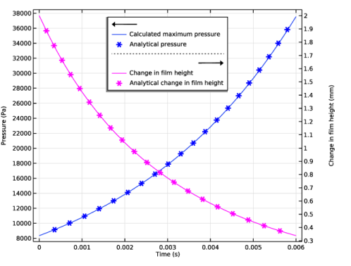
In the Settings window for 1D Plot Group, type Maximum Pressure and Change in Film Height in the Label text field.
3
Click to expand the Title section. From the Title type list, choose None.
4
Locate the Plot Settings section. Select the Two y-axes checkbox.
5
In the table, select the Plot on secondary y-axis checkboxes for Global 1 and Global 2.
6
Select the y-axis label checkbox. In the associated text field, type Pressure (Pa).
7
Select the Secondary y-axis label checkbox.
8
Locate the Legend section. From the Position list, choose Upper middle.
9
In the Maximum Pressure and Change in Film Height toolbar, click  Plot.