PDF

Oil–Water Flow Through an Orifice — A Droplet Population Model
Introduction
This example considers the turbulent flow of an oil–water suspension through an orifice. The oil droplets are broken up into smaller droplets by the turbulent stresses as the suspension passes through the orifice. The aim of this model is to track the distribution of droplet sizes. The droplet size distribution is discretized into five populations of droplets with different diameters. The model uses the Phase Transport Mixture Model, Turbulent Flow, k-ε multiphysics interface, to compute the flow field and the transport of the different droplet populations.
Model Definition
The oil–water suspension flows through a pipe with a radius of 5 cm. The pipe contains an orifice with a radius of 1 cm. The section of the pipe that is taken to be the model geometry is 60 cm long, and the orifice is located 15 cm from the inlet boundary. The flow is assumed to be axially symmetric. See Figure 1 below for a graphic representation of the geometry.
Figure 1: Cross section of the axially symmetric model geometry, which consists of a pipe with an orifice.
The stationary flow field for the mixture is computed using the Turbulent Flow, k-ε interface. The Mixture Model multiphysics coupling node computes from the mixture flow field the velocity fields of the dispersed phases. These dispersed phase velocity fields are used for the transport of the droplet populations in the Phase Transport interface which in this case is set up to solve for the volume fractions si of five different droplet sizes (diameters). The diameters in the populations with volume fraction s1, …, s5 are chosen to be d0/4, d0/2,d0, 2d0, and 4d0, respectively, where the diameter d0 is an input to the model. The diameter d0 is taken to be 0.5 mm in this case.
The droplet break-up is modeled as follows: the maximum stable droplet size dmax is estimated using the relation
(1)
where σ denotes the surface tension (taken to be 0.03 N/m), ρc the density of the continuous phase, and ε the energy dissipation rate of the flow. This relation can be derived (see Ref. 1) by assuming that a droplet will break up when the droplet Weber number is larger than a critical Weber number. The Weber number for a droplet with diameter d is defined by
(2)
Here Δu is the difference of the flow velocity across the droplet. Using the relation
(3)
between Δu and ε, which is valid under the assumption of homogeneous isotropic turbulence, and setting the critical Weber number to 1, the relation in Equation 1 now follows. To derive an expression for the droplet break-up rate, it is assumed that the droplet break-up rate of the population of droplets with diameter di is inversely proportional to the turbulent dissipation time τ and proportional to the relative difference between the volumes (di)3/(6π) and (dmax)3/(6π), whenever di is larger than dmax. This leads to a mass sink in the conservation equation for the population of droplets with diameter di of the form
(4)
where ρd is the density of the dispersed phase. As mass is conserved, as coalescence is not taken into account, and as it is assumed that droplets of diameter di break up into droplets with diameter di1 = di/2, the total mass source for the population of droplets with diameter di is given by
(5)
In addition R1 and R6 are taken to be zero: the smallest droplets do not break up into even smaller droplets, and there are no larger droplets that break up into droplets with diameter 4d0.
The density and viscosity of the continuous and dispersed phases are taken from the Water, liquid and Transformer oil materials from COMSOL’s material databases.
The flow field is solved for three different values of the inflow velocity, which are computed from three different total mass flow rates: 1 kg/s, 5 kg/s, and 10 kg/s. The volume fraction of the dispersed phase at the inlet is 0.05, which is distributed over the inlet volume fractions si0 of the different droplet populations as follows:
(6)
where the xi are the fractions of the total inlet number density, given by x1 = x5 = 0.1, x2 = x4 = 0.2, and x3 = 0.4.
Figure 2: The magnitude of the volume-averaged velocity field of the mixture for a mass flow rate of 5 kg/s.
Results and Discussion
In Figure 2 the magnitude of the volume-averaged velocity field of the mixture is plotted for a mass flow rate of 5 kg/s. It can be seen that the oil–water mixture accelerates as it passes through the orifice, and the flow becomes more turbulent. There are no mass sources for the dispersed phase in the system, so the overall volume fraction of the oil droplets stays more or less constant throughout the pipe. However, due to turbulent stresses the volume fractions of the individual droplet populations change considerably as the mixture flows through the pipe.
.
Figure 3: The volume fractions of the five droplet populations along the centerline of the pipe for a mass flow rate of 1 kg/s. The average oil droplet size decreases as the water-oil mixture flows through the orifice.
In Figure 3 the volume fractions of the five droplet populations are plotted along the centerline of the pipe for a mass flow rate of 1 kg/s. The plot shows that the droplet size distribution does not change until the mixture reaches the orifice. When the mixture does reach the orifice, the volume fraction of the population with the largest droplets starts to decrease, indicating that the largest droplets break up into smaller ones, and it decreases until all the largest droplets are broken up. Similarly, the population of the second largest droplets decreases as the mixture passes through the orifice. The populations with the three smallest droplet sizes, however, all increase. This means that, as is expected, the average oil droplet size has decreased after the mixture has passed through the orifice. For higher mass flow rates, it is expected that the average droplet size will decrease even further. Figure 4, which shows the population volume fractions for a mass flow rate of 10 kg/s, illustrates that this is indeed the case: the volume fractions of all droplet populations vanish as the mixture flows through the orifice, except for the population with the smallest droplets.
Figure 4: The volume fractions of the five droplet populations along the centerline of the pipe for a mass flow rate of 10 kg/s. Only the population with the smallest droplet size remains after the orifice.
Reference
1. M.J. van der Zande and W.M.G.T. van den Broek, The Effect of Tubing and Choke Valve on Oil-Droplet Break-up, proceedings of the 1st North American Conference on Multiphase Technology, Banff, Canada, June 10–11, 1998, pp. 89–100.
Application Library path: CFD_Module/Multiphase_Flow/droplet_population_model
Modeling Instructions
From the File menu, choose New.
New
In the New window, click  Model Wizard.
Model Wizard
1
In the Model Wizard window, click  2D Axisymmetric.
2
In the Select Physics tree, select Fluid Flow > Multiphase Flow > Phase Transport Mixture Model > Turbulent Flow > Turbulent Flow, k-ε.
3
Click Add.
4
Click  Study.
5
In the Select Study tree, select General Studies > Stationary.
6
Global Definitions
Parameters 1
1
In the Model Builder window, under Global Definitions click Parameters 1.
2
In the Settings window for Parameters, locate the Parameters section.
3
Click  Load from File.
4
Definitions
Variables 1
1
In the Definitions toolbar, click  Local Variables.
2
In the Settings window for Variables, locate the Variables section.
3
Click  Load from File.
4
Geometry 1
Rectangle 1 (r1)
1
In the Geometry toolbar, click  Rectangle.
2
In the Settings window for Rectangle, locate the Size and Shape section.
3
In the Width text field, type r_pipe.
4
In the Height text field, type h_pipe.
Rectangle 2 (r2)
1
In the Geometry toolbar, click  Rectangle.
2
In the Settings window for Rectangle, locate the Size and Shape section.
3
In the Width text field, type r_pipe-r_orifice.
4
In the Height text field, type h_orifice.
5
Locate the Position section. In the r text field, type r_orifice.
6
In the z text field, type h_orifice_pos.
Difference 1 (dif1)
1
In the Geometry toolbar, click  Booleans and Partitions and choose Difference.
2
3
In the Settings window for Difference, locate the Difference section.
4
Click to select the  Activate Selection toggle button for Objects to subtract.
5
Fillet 1 (fil1)
1
In the Geometry toolbar, click  Fillet.
2
On the object dif1, select Points 3 and 4 only.
3
In the Settings window for Fillet, locate the Radius section.
4
In the Radius text field, type 0.003.
5
Click  Build All Objects.
Add Material
1
In the Materials toolbar, click  Add Material to open the Add Material window.
2
Go to the Add Material window.
3
In the tree, select Built-in > Water, liquid.
4
Click the Add to Component button in the window toolbar.
5
In the tree, select Liquids and Gases > Liquids > Transformer oil.
6
Click the Add to Component button in the window toolbar.
7
In the Materials toolbar, click  Add Material to close the Add Material window.
Materials
Transformer oil (mat2)
Select Domain 1 only.
Turbulent Flow, k-ε (spf)
1
In the Model Builder window, under Component 1 (comp1) click Turbulent Flow, k-ε (spf).
2
In the Settings window for Turbulent Flow, k-ε, locate the Physical Model section.
3
Select the Include gravity checkbox.
Initial Values 1
1
In the Model Builder window, under Component 1 (comp1) > Turbulent Flow, k-ε (spf) click Initial Values 1.
2
In the Settings window for Initial Values, locate the Initial Values section.
3
Specify the u vector as
Inlet 1
1
In the Physics toolbar, click  Boundaries and choose Inlet.
2
3
In the Settings window for Inlet, locate the Velocity section.
4
In the U0 text field, type u_0.
Outlet 1
1
In the Physics toolbar, click  Boundaries and choose Outlet.
2
Phase Transport (phtr)
1
In the Model Builder window, under Component 1 (comp1) click Phase Transport (phtr).
2
In the Settings window for Phase Transport, click to expand the Dependent Variables section.
3
In the Number of phases text field, type 6.
4
Locate the Phases section. From the From volume constraint list, choose s6.
Initial Values 1
1
In the Model Builder window, under Component 1 (comp1) > Phase Transport (phtr) click Initial Values 1.
2
In the Settings window for Initial Values, locate the Initial Values section.
3
In the s0,s1 text field, type s1_0. Similarly, type s2_0, s3_0, s4_0, and s5_0, respectively, in the next text fields.
Mass Source 1
1
In the Physics toolbar, click  Domains and choose Mass Source.
2
3
In the Settings window for Mass Source, locate the Mass Source section.
4
In the Qs1 text field, type R2.
5
In the Qs2 text field, type R3-R2.
6
In the Qs3 text field, type R4-R3.
7
In the Qs4 text field, type R5-R4.
8
In the Qs5 text field, type -R5.
Outflow 1
1
In the Physics toolbar, click  Boundaries and choose Outflow.
2
Volume Fraction 1
1
In the Physics toolbar, click  Boundaries and choose Volume Fraction.
2
3
In the Settings window for Volume Fraction, locate the Volume Fraction section.
4
Select the Phase s1 checkbox.
5
In the s0,s1 text field, type s1_0.
6
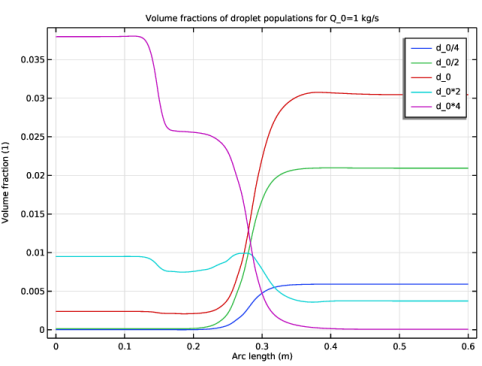
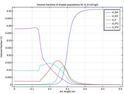
Repeat the last two steps for the remaining phases: select the checkboxes, and type s2_0, s3_0, s4_0, and s5_0, respectively, in the text fields.
Multiphysics
Mixture Model 1 (mfmm1)
1
In the Model Builder window, under Component 1 (comp1) > Multiphysics click Mixture Model 1 (mfmm1).
2
In the Settings window for Mixture Model, locate the Physical Model section.
3
From the Dispersed phase list, choose Liquid droplets/bubbles.
4
From the Slip model list, choose Schiller–Naumann.
5
From the Mixture viscosity model list, choose Volume averaged.
6
Locate the Continuous Phase Properties section. From the Continuous phase list, choose Water, liquid (mat1).
7
Locate the Dispersed Phase 1 Properties section. From the Phase s1 list, choose Transformer oil (mat2).
8
In the ds1 text field, type d_0/4.
9
Mesh 1
1
In the Model Builder window, under Component 1 (comp1) click Mesh 1.
2
In the Settings window for Mesh, locate the Physics-Controlled Mesh section.
3
From the Element size list, choose Fine.
Study 1
Step 1: Stationary
1
In the Model Builder window, under Study 1 click Step 1: Stationary.
2
In the Settings window for Stationary, click to expand the Study Extensions section.
3
Select the Auxiliary sweep checkbox.
4
5
6
In the Study toolbar, click  Compute.
Results
Volume Fractions along Centerline
1
In the Results toolbar, click  1D Plot Group.
2
Right-click 1D Plot Group 7 and choose Rename.
3
In the Rename 1D Plot Group dialog, type Volume Fractions along Centerline in the New label text field.
4
5
In the Settings window for 1D Plot Group, locate the Data section.
6
From the Parameter selection (Q_0) list, choose From list.
7
In the Parameter values (Q_0 (kg/s)) list box, select 1.
8
Click to expand the Title section. From the Title type list, choose Manual.
9
In the Title text area, type Volume fractions of droplet populations for Q_0=1 kg/s.
Line Graph 1
1
In the Volume Fractions along Centerline toolbar, click  Line Graph.
2
3
In the Settings window for Line Graph, locate the y-Axis Data section.
4
In the Expression text field, type s1.
5
Click to expand the Legends section. Select the Show legends checkbox.
6
From the Legends list, choose Manual.
7
Line Graph 2
1
Right-click Line Graph 1 and choose Duplicate.
2
In the Settings window for Line Graph, locate the y-Axis Data section.
3
In the Expression text field, type s2.
4
Locate the Legends section. In the table, enter the following settings:
Line Graph 3-5
Repeat the four previous instructions for the remaining three phases: duplicate the previous line graph, set the Expression text field in the y-Axis Data section to s3_0, s4_0, and s5_0, respectively, and change the settings for the legends accordingly. And then, as a final step to produce Figure 3:
Line Graph 3
1
In the Model Builder window, click Line Graph 3.
2
In the Volume Fractions along Centerline toolbar, click  Plot.
Velocity (spf)
The following instructions create the plot that is used as the model thumbnail.
Revolution 2D 2
1
In the Model Builder window, expand the Results > Datasets node.
2
Right-click Revolution 2D and choose Duplicate.
Selection
1
In the Results toolbar, click  Attributes and choose Selection.
2
In the Settings window for Selection, locate the Geometric Entity Selection section.
3
From the Geometric entity level list, choose Boundary.
4
Surface
1
In the Model Builder window, expand the Results > Velocity, 3D (spf) node, then click Surface.
2
In the Settings window for Surface, locate the Coloring and Style section.
3
From the Coloring list, choose Uniform.
4
From the Color list, choose Gray.
5
Click to expand the Title section. From the Title type list, choose None.
6
Locate the Data section. From the Dataset list, choose Revolution 2D 2.
Streamline 1
1
In the Model Builder window, right-click Velocity, 3D (spf) and choose Streamline.
2
In the Settings window for Streamline, locate the Streamline Positioning section.
3
In the Points text field, type 40.
4
Locate the Coloring and Style section. Find the Line style subsection. From the Type list, choose Tube.
Color Expression 1
1
Right-click Streamline 1 and choose Color Expression.
2
In the Settings window for Color Expression, locate the Coloring and Style section.
3
From the Color table list, choose Cividis.
4
From the Color table transformation list, choose Reverse.