|
|
|

|
1
|
|
2
|
|
3
|
Click Add.
|
|
4
|
Click
|
|
5
|
|
6
|
Click
|
|
1
|
|
2
|
|
1
|
|
2
|
|
3
|
|
4
|
|
5
|
|
6
|
Click to expand the Layers section. In the table, enter the following settings:
|
|
7
|
|
8
|
Clear the Bottom checkbox.
|
|
1
|
|
2
|
|
3
|
|
4
|
|
5
|
|
6
|
|
7
|
|
1
|
|
2
|
|
3
|
|
4
|
|
5
|
|
6
|
|
7
|
|
8
|
|
1
|
|
2
|
On the object cyl1, select Point 2 only.
|
|
3
|
|
4
|
|
5
|
On the object blk2, select Point 5 only.
|
|
1
|
|
2
|
On the object cyl1, select Point 6 only.
|
|
3
|
|
4
|
|
5
|
On the object blk2, select Point 7 only.
|
|
1
|
|
2
|
On the object cyl1, select Point 8 only.
|
|
3
|
|
4
|
|
5
|
On the object blk2, select Point 8 only.
|
|
1
|
|
2
|
On the object cyl1, select Point 4 only.
|
|
3
|
|
4
|
|
5
|
On the object blk2, select Point 6 only.
|
|
6
|
Click
|
|
7
|
Click the
|
|
1
|
|
2
|
|
3
|
|
4
|
|
5
|
Select the object cyl1 only.
|
|
6
|
|
7
|
|
8
|
|
1
|
|
2
|
On the object fin, select Domains 2, 4, and 5 only.
|
|
1
|
|
2
|
On the object mcd1, select Edges 9, 10, 22, and 24 only.
|
|
3
|
|
1
|
|
2
|
|
3
|
|
4
|
Select the Group by continuous tangent checkbox.
|
|
6
|
|
1
|
|
2
|
In the Show More Options dialog, in the tree, select the checkbox for the node Physics > Stabilization.
|
|
3
|
Click OK.
|
|
4
|
|
5
|
|
6
|
|
7
|
Click to expand the Discretization section. From the Discretization of fluids list, choose P2+P2. P2+P2 is used because it is more conservative and more accurate than P2+P1 and P1+P1.
|
|
1
|
In the Model Builder window, under Component 1 (comp1) > Laminar Flow (spf) click Fluid Properties 1.
|
|
2
|
|
3
|
|
4
|
|
1
|
|
3
|
|
4
|
In the U0 text field, type 36*U_mean*z*y*(H-y)*(H-z)/H^4*sin(pi*t/8[s]), which corresponds to Equation 1.
|
|
1
|
|
1
|
|
2
|
|
3
|
|
4
|
|
1
|
|
2
|
|
1
|
|
2
|
In the Settings window for Interpolation, type Interpolation: Reference Lift Coefficient in the Label text field.
|
|
3
|
|
4
|
|
5
|
Click
|
|
6
|
Browse to the model’s Application Libraries folder and double-click the file cylinder_flow_3d_periodic_LiftRef.txt.
|
|
7
|
Locate the Data Column Settings section. In the table, click to select the cell at row number 1 and column number 1.
|
|
8
|
|
1
|
|
2
|
In the Settings window for Interpolation, type Interpolation: Reference Drag Coefficient in the Label text field.
|
|
3
|
|
4
|
|
5
|
Click
|
|
6
|
Browse to the model’s Application Libraries folder and double-click the file cylinder_flow_3d_periodic_DragRef.txt.
|
|
7
|
Locate the Data Column Settings section. In the table, click to select the cell at row number 1 and column number 1.
|
|
8
|
|
1
|
|
2
|
|
3
|
|
4
|
|
1
|
|
1
|
|
1
|
|
3
|
|
4
|
|
5
|
|
6
|
|
1
|
|
3
|
|
4
|
|
5
|
|
6
|
|
7
|
Click
|
|
1
|
|
1
|
|
1
|
|
3
|
|
4
|
|
5
|
|
6
|
|
7
|
|
8
|
Select the Reverse direction checkbox.
|
|
1
|
|
3
|
|
4
|
|
5
|
|
6
|
|
7
|
|
8
|
Click
|
|
1
|
|
1
|
|
3
|
|
4
|
|
5
|
|
6
|
|
1
|
|
3
|
|
4
|
|
5
|
|
6
|
|
1
|
|
3
|
|
4
|
|
5
|
|
6
|
|
7
|
|
8
|
Click
|
|
1
|
|
2
|
|
3
|
|
4
|
|
5
|
|
6
|
|
7
|
Select the Symmetric distribution checkbox.
|
|
8
|
Click
|
|
1
|
|
2
|
|
3
|
|
4
|
|
5
|
|
1
|
|
2
|
|
3
|
In the Model Builder window, under Study 1 > Solver Configurations > Solution 1 (sol1) click Time-Dependent Solver 1.
|
|
4
|
|
5
|
|
6
|
|
7
|
|
8
|
|
1
|
|
2
|
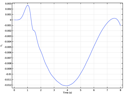
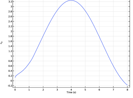
In the Settings window for Global Evaluation, type Global Evaluation: Lift and Drag Coefficients in the Label text field.
|
|
3
|
Locate the Expressions section. In the table, enter the following settings:
|
|
4
|
Click
|
|
1
|
|
2
|
|
1
|
Go to the Table 1: Lift and Drag Coefficients window.
|
|
2
|
Click the Table Graph button in the window toolbar.
|
|
1
|
|
2
|
|
3
|
|
1
|
|
2
|
|
3
|
Locate the Plot Settings section.
|
|
4
|
|
1
|
|
2
|
|
3
|
|
4
|
|
5
|
|
1
|
|
2
|
|
3
|
|
1
|
In the Model Builder window, right-click Global Evaluation: Lift and Drag Coefficients and choose Duplicate.
|
|
2
|
In the Settings window for Global Evaluation, type Global Evaluation: Maximum Lift and Drag Coefficients in the Label text field.
|
|
3
|
|
4
|
|
1
|
|
2
|
In the Settings window for Global Evaluation, type Global Evaluation: Minimum Lift and Drag Coefficients in the Label text field.
|
|
3
|
|
4
|
|
1
|
|
2
|
In the Settings window for Table, type Table 2: Maximum Lift and Drag Coefficients in the Label text field.
|
|
1
|
|
2
|
In the Settings window for Table, type Table 3: Minimum Lift and Drag Coefficients in the Label text field.
|
|
1
|
|
2
|
|
4
|
|
5
|
|
6
|
|
1
|
|
2
|
|
1
|
|
2
|
|
3
|
Clear the Show legends checkbox.
|
|
4
|
|
5
|
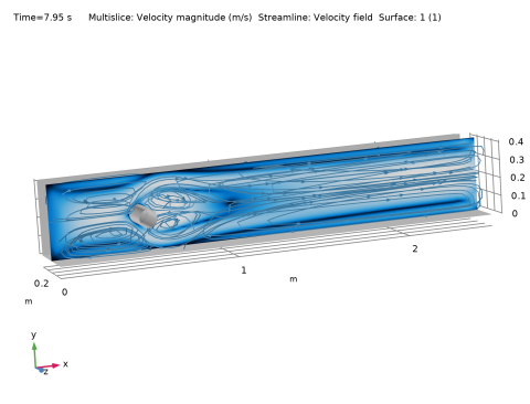
Locate the Data section. From the Time (s) list, choose 7.95. Since the inlet velocity vanishes at the final time step, the solution at t=7.95s is chosen for a better visualization of the streamlines.
|
|
1
|
|
2
|
|
3
|
|
4
|
|
5
|
|
1
|
|
2
|
|
3
|
|
4
|
|
5
|
Locate the Coloring and Style section. Find the Line style subsection. From the Type list, choose Tube.
|
|
6
|
|
7
|
|
8
|
|
9
|
|
10
|
Click Define custom colors.
|
|
12
|
Click Add to custom colors.
|
|
13
|
|
1
|
|
2
|
|
3
|
|
4
|
|
5
|
|
1
|
|
2
|
|
3
|
From the Selection list, choose Cylinder, and add the bottom and back boundaries. This corresponds to:
|
|
5
|