|
|
|


|
1
|
|
2
|
In the Select Physics tree, select Electrochemistry > Batteries > Battery with Binary Electrolyte (batbe).
|
|
3
|
Click Add.
|
|
4
|
Click
|
|
5
|
|
6
|
Click
|
|
1
|
|
2
|
|
3
|
Click
|
|
4
|
Browse to the model’s Application Libraries folder and double-click the file zn_ago_battery_1d_parameters.txt.
|
|
1
|
|
2
|
|
3
|
Click
|
|
4
|
Browse to the model’s Application Libraries folder and double-click the file zn_ago_battery_1d_variables.txt.
|
|
1
|
|
2
|
|
3
|
|
5
|
|
1
|
In the Model Builder window, under Component 1 (comp1) click Battery with Binary Electrolyte (batbe).
|
|
2
|
In the Settings window for Battery with Binary Electrolyte, locate the Cross-Sectional Area section.
|
|
3
|
|
4
|
|
5
|
|
6
|
|
1
|
In the Model Builder window, under Component 1 (comp1) > Battery with Binary Electrolyte (batbe) click Separator 1.
|
|
2
|
|
3
|
|
4
|
|
5
|
|
6
|
|
7
|
|
8
|
|
9
|
Locate the Effective Transport Parameter Correction section. From the Electrolyte conductivity list, choose No correction.
|
|
1
|
|
2
|
In the Settings window for Porous Electrode, type Porous Electrode: AgO (positive electrode) in the Label text field.
|
|
4
|
Locate the Electrolyte Properties section. From the σl list, choose User defined. In the associated text field, type sigmaleff.
|
|
5
|
|
6
|
|
7
|
|
8
|
|
9
|
|
10
|
|
11
|
|
12
|
|
13
|
Locate the Effective Transport Parameter Correction section. From the Electrolyte conductivity list, choose No correction.
|
|
14
|
|
15
|
|
17
|
Click
|
|
19
|
Click
|
|
1
|
|
2
|
|
3
|
|
4
|
|
5
|
|
6
|
|
7
|
Locate the Electrode Kinetics section. From the Kinetics expression type list, choose Butler–Volmer.
|
|
8
|
|
9
|
|
10
|
|
11
|
Locate the Active Specific Surface Area section. From the Active specific surface area list, choose User defined. In the av text field, type a.
|
|
12
|
|
13
|
In the Stoichiometric coefficients for dissolving–depositing species: table, enter the following settings:
|
|
14
|
|
1
|
In the Physics toolbar, click
|
|
2
|
In the Settings window for Initial Values for Dissolving–Depositing Species, locate the Initial Values for Dissolving–Depositing Species section.
|
|
1
|
|
2
|
In the Settings window for Porous Electrode, type Porous Electrode: Zn (negative electrode) in the Label text field.
|
|
4
|
Locate the Electrolyte Properties section. From the σl list, choose User defined. In the associated text field, type sigmaleff.
|
|
5
|
|
6
|
|
7
|
|
8
|
|
9
|
|
10
|
|
11
|
|
12
|
|
13
|
Locate the Effective Transport Parameter Correction section. From the Electrolyte conductivity list, choose No correction.
|
|
14
|
|
15
|
|
17
|
Click
|
|
1
|
|
2
|
|
3
|
|
4
|
|
5
|
|
6
|
|
7
|
Locate the Electrode Kinetics section. From the Kinetics expression type list, choose Butler–Volmer.
|
|
8
|
|
9
|
|
10
|
|
11
|
Locate the Active Specific Surface Area section. From the Active specific surface area list, choose User defined. In the av text field, type a.
|
|
12
|
|
13
|
In the Stoichiometric coefficients for dissolving–depositing species: table, enter the following settings:
|
|
14
|
|
1
|
In the Physics toolbar, click
|
|
2
|
In the Settings window for Initial Values for Dissolving–Depositing Species, locate the Initial Values for Dissolving–Depositing Species section.
|
|
1
|
|
1
|
|
3
|
|
4
|
From the list, choose Galvanostatic.
|
|
5
|
|
6
|
|
7
|
|
1
|
|
2
|
|
3
|
|
4
|
|
5
|
|
6
|
Click
|
|
7
|
Browse to the model’s Application Libraries folder and double-click the file zn_ago_battery_1d_pulse.txt.
|
|
1
|
In the Model Builder window, under Component 1 (comp1) > Battery with Binary Electrolyte (batbe) click Initial Values 1.
|
|
2
|
|
3
|
|
4
|
|
5
|
|
1
|
|
3
|
|
4
|
|
5
|
|
1
|
|
2
|
|
3
|
|
4
|
|
1
|
|
2
|
|
3
|
Click
|
|
1
|
|
2
|
|
3
|
|
1
|
|
2
|
|
3
|
In the Model Builder window, expand the Study 1 > Solver Configurations > Solution 1 (sol1) > Dependent Variables 1 node, then click Dissolving–Depositing Species Concentration (comp1.batbe.pce1.c).
|
|
4
|
|
5
|
|
6
|
|
7
|
In the Model Builder window, under Study 1 > Solver Configurations > Solution 1 (sol1) > Dependent Variables 1 click Dissolving–Depositing Species Concentration (comp1.batbe.pce2.c).
|
|
8
|
|
9
|
|
10
|
|
11
|
In the Model Builder window, under Study 1 > Solver Configurations > Solution 1 (sol1) click Time-Dependent Solver 1.
|
|
12
|
|
13
|
|
14
|
|
15
|
|
16
|
Clear the Generate default plots checkbox.
|
|
17
|
|
1
|
|
2
|
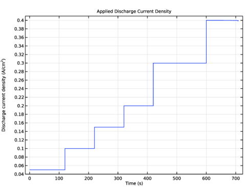
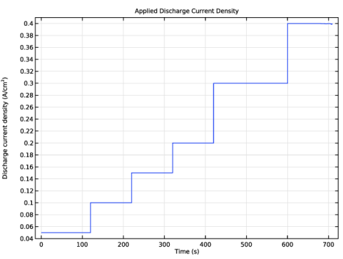
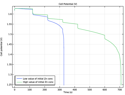
In the Settings window for 1D Plot Group, type Applied Discharge Current Density in the Label text field.
|
|
1
|
|
3
|
In the Settings window for Point Graph, click Replace Expression in the upper-right corner of the y-Axis Data section. From the menu, choose Component 1 (comp1) > Battery with Binary Electrolyte > batbe.nIs - Normal electrode current density - A/m².
|
|
4
|
|
1
|
|
2
|
|
3
|
|
4
|
Locate the Plot Settings section.
|
|
5
|
Select the y-axis label checkbox. In the associated text field, type Discharge current density (A/cm<sup>2</sup>).
|
|
6
|
|
1
|
|
2
|
|
3
|
|
1
|
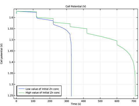
In the Model Builder window, expand the Applied Discharge Current Density 1 node, then click Results > Cell Potential (V) > Point Graph 1.
|
|
2
|
In the Settings window for Point Graph, click Replace Expression in the upper-right corner of the y-Axis Data section. From the menu, choose Component 1 (comp1) > Battery with Binary Electrolyte > phis - Electric potential - V.
|
|
3
|
|
4
|
|
1
|
|
2
|
|
3
|
|
4
|
|
5
|
|
1
|
|
2
|
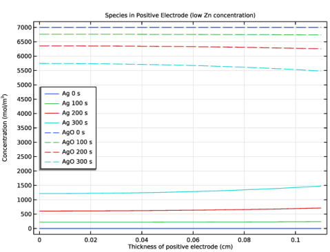
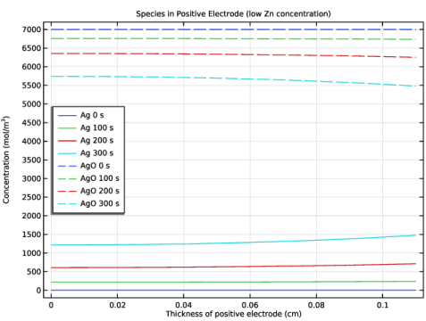
In the Settings window for 1D Plot Group, type Species in Positive Electrode (low Zn concentration) in the Label text field.
|
|
3
|
|
4
|
|
5
|
|
6
|
|
1
|
|
3
|
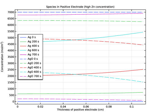
In the Settings window for Line Graph, click Replace Expression in the upper-right corner of the y-Axis Data section. From the menu, choose Component 1 (comp1) > Definitions > Variables > cAg - Concentration of Ag - mol/m³.
|
|
4
|
|
5
|
|
6
|
|
7
|
|
8
|
|
9
|
|
1
|
|
2
|
In the Settings window for Line Graph, click Replace Expression in the upper-right corner of the y-Axis Data section. From the menu, choose Component 1 (comp1) > Definitions > Variables > cAgO - Concentration of AgO - mol/m³.
|
|
3
|
|
4
|
|
5
|
|
6
|
|
1
|
|
2
|
|
3
|
|
4
|
Locate the Plot Settings section.
|
|
5
|
Select the x-axis label checkbox. In the associated text field, type Thickness of positive electrode (cm).
|
|
6
|
Select the y-axis label checkbox. In the associated text field, type Concentration (mol/m<sup>3</sup>).
|
|
7
|
|
8
|
|
1
|
|
2
|
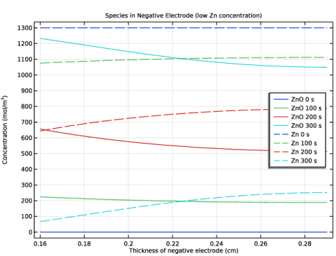
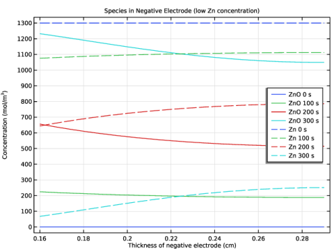
In the Settings window for 1D Plot Group, type Species in Negative Electrode (low Zn concentration) in the Label text field.
|
|
3
|
|
4
|
|
5
|
|
6
|
|
1
|
|
3
|
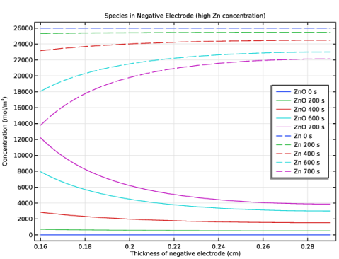
In the Settings window for Line Graph, click Replace Expression in the upper-right corner of the y-Axis Data section. From the menu, choose Component 1 (comp1) > Definitions > Variables > cZnO - Concentration of ZnO - mol/m³.
|
|
4
|
|
5
|
|
6
|
|
7
|
|
8
|
|
9
|
|
1
|
|
2
|
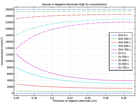
In the Settings window for Line Graph, click Replace Expression in the upper-right corner of the y-Axis Data section. From the menu, choose Component 1 (comp1) > Definitions > Variables > cZn - Concentration of Zn - mol/m³.
|
|
3
|
Locate the Coloring and Style section. Find the Line style subsection. From the Line list, choose Dashed.
|
|
4
|
|
5
|
|
1
|
|
2
|
|
3
|
|
4
|
Locate the Plot Settings section.
|
|
5
|
Select the x-axis label checkbox. In the associated text field, type Thickness of negative electrode (cm).
|
|
6
|
Select the y-axis label checkbox. In the associated text field, type Concentration (mol/m<sup>3</sup>).
|
|
7
|
|
8
|
|
1
|
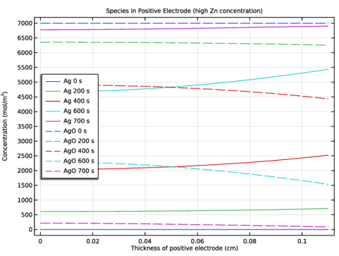
In the Model Builder window, right-click Species in Positive Electrode (low Zn concentration) and choose Duplicate.
|
|
2
|
In the Settings window for 1D Plot Group, type Species in Positive Electrode (high Zn concentration) in the Label text field.
|
|
3
|
|
4
|
|
5
|
|
1
|
In the Model Builder window, right-click Species in Negative Electrode (low Zn concentration) and choose Duplicate.
|
|
2
|
In the Settings window for 1D Plot Group, type Species in Negative Electrode (high Zn concentration) in the Label text field.
|
|
3
|
|
4
|
|
5
|