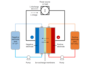
PDF

Vanadium Redox Flow Battery
Introduction
Redox flow batteries store energy in the liquid electrolytes, pumped through the cell and stored in external tanks, rather than in the porous electrodes like conventional batteries. This approach offers interesting solutions for low-cost energy storage, load leveling, and power peak shaving.
The vanadium redox flow battery uses two different electrolyte solutions, one for the negative side of the cell and another for the positive side. The two solutions are kept separated in the cell by the use of an ion-exchange membrane that allows for transport of ions (primarily protons) between the two cell compartments. The principle of the vanadium redox flow battery is illustrated in Figure 1.
Figure 1: Schematic of a vanadium redox flow battery system.
This example demonstrates how to build a model consisting of two different cell compartments, with different ion compositions and electrode reactions, separated by an ion-exchange membrane. The model is a modified version of published works (Ref. 1 and Ref. 2).
See also the Application Libraries example Soluble Lead–Acid Redox Flow Battery for how to make a transient flow battery model by coupling the cell model to mass balances for the external storage tanks.
Model Definition
The cell geometry is shown in Figure 2. The model contains three domains, a negative porous electrode (4 mm thick), an ion-exchange membrane (203 μm thick) and a positive porous electrode (4 mm thick). The cell is 35 mm high.
Figure 2: Model geometry. Three domains: negative electrode, membrane, positive electrode.
Each side of the cell is fed with an electrolyte containing sulfuric acid and a vanadium redox couple (see below), flowing through the porous electrodes. The liquid enters the cell from the bottom at a constant velocity in the y direction, corresponding to a flow rate of 30 ml/min at a cell depth of 28.5 mm.
The left electrode is grounded, and the current leaves the cell over the rightmost boundary at an average current density of 100 mA/cm2.
The models solves for a stationary case with a given set of inlet concentrations.
Liquid Electrolyte Species and Electrode Reactions
The negative electrolyte contains the following ions:
H+
HSO4-
SO42-
V3+
V2+
The negative electrode reaction is
The equilibrium potential for this reaction is calculated using Nernst equation according to
where E0,neg is the reference potential for the electrode reaction (SI unit: V), ai is the chemical activity of species i (dimensionless), R is the molar gas constant (8.31 J/(mol·K)), T is the cell temperature (SI unit: K), and F is Faraday’s constant (96,485 s·A/mol).
A Butler–Volmer type of kinetics expression is used for the negative electrode reaction according to:
where A is the specific surface area (SI unit: m2/m3) of the porous electrode, αneg the transfer coefficient (dimensionless), and kneg the rate constant.
The overpotential, ηneg (SI unit: V), is defined as
where ϕs is the electric potential of the solid phase of the electrode (SI unit: V) and ϕl the electrolyte potential (SI unit: V).
The positive electrolyte contains the following ions:
H+
HSO4-
SO42-
VO2+
VO2+
The positive electrode reaction is
with the equilibrium potential calculated according to
The ion-exchange membrane accounts for transport of the following ions:
H+
HSO4-
SO42-
V3+
V2+
VO2+
VO2+
Sulfuric Acid Dissociation
The first dissociation step of sulfuric acid is assumed to be complete
whereas the second step
is described using a dissociation source term, rd:
where kd is a rate parameter, and β the degree of dissociation.
Ion Transport Equations
In this model the Nernst–Planck equations are used for ion flux and charge transport. The following equation describes the molar flux of species i, Ni, due to diffusion, migration, and convection:
The first term is the diffusion flux and Di is the diffusion coefficient (SI unit: m2/s). The migration term consists of the species charge number zi, the species mobility umob,i (SI unit: s·mol/kg) and the electrolyte potential (ϕl). In the convection term, u denotes the fluid velocity vector (SI unit: m/s).
The electrolyte current density is calculated using Faraday’s law by summing up the contributions from the molar fluxes, multiplied by the species charges, with the observation that the convective term vanishes due to the electroneutrality condition (see the theory for the Tertiary Current Distribution, Nernst–Planck interface):
(1)
The conservation of charge is then used to calculate the electrolyte potential.
where the Ri terms are the reaction sources due the porous electrode reactions.
This model uses Equation 1 when solving for the electrolyte potential in the porous electrodes through the Tertiary Current Distribution, Nernst–Planck interface.
In the negative and positive porous electrode domains, where there is free electrolyte present, the concentrations for all the ions are of the same order of magnitude, and the gradients of ci are not negligible. The membrane, however, consists of a polymer electrolyte, with additional negative ions fixed in the polymer matrix, implying that the concentration for this species is constant. In the ion-exchange membrane domain, a fixed space charge, ρfix, is added while calculating the sum of charges in the electroneutrality condition:
(2)
The fixed space charge is prescribed in terms of the membrane charge concentration.
The checkbox Add Donnan shift to initial values, when enabled, shifts the initial values on the selection of the Ion-Exchange Membrane node in order to fulfill electroneutrality and compliance with the Donnan equilibria.
Membrane — Porous Electrode Boundary Conditions
Donnan Conditions
The boundary conditions at the boundaries between the membrane and the porous electrode domains are set up as follows.
For species existing on both sides of the membrane-electrode, we have the following relation between the potentials and the concentrations:
(3)
where ci,m is the species concentration in the membrane, and ci,e the species concentration in the free electrolyte and zi the corresponding charge. The potential shift caused by Equation 3 is called Donnan potential (Ref. 3). The Ion-Exchange Membrane Boundary feature in the Tertiary Current Distribution, Nernst–Planck interface is used to define the Donnan conditions.
Self-discharge Reactions
At the membrane-positive electrode boundary, the V3+ and V2+ are assumed to be immediately oxidized according to
and
so that
(4)
Correspondingly, the VO2+ and VO2+ concentrations are assumed to be zero at the membrane–negative electrode boundaries:
(5)
as a result of the reduction reactions
and
the fast oxidation/reduction reactions are implemented using the Fast Irreversible Reaction kinetics type of the Electrode Surface node.
Results and Discussion
Figure 3 shows the concentration of the V3+ and the VO2+ ions in the porous electrodes for a membrane negative charge concentration of 1990 mol/m3. The ion concentrations of these species are higher toward the current collectors and toward the outlets.
Figure 3: Concentration (mol/m3) of the V3+ (left compartment) and the VO2+ (right compartment) ions for a membrane negative charge concentration of 1990 mol/m3.
Figure 4 shows the concentration of the V2+ and the VO2+ ions for the membrane negative charge concentration of 1990 mol/m3. Depletion occurs along the flow direction and also toward both the current collector and membrane sides of the electrodes.
Figure 4: Concentration (mol/m3) of the V2+ (left compartment) and the VO2+ (right compartment) ions for a membrane negative charge concentration of 1990 mol/m3.
Figure 5 shows the electrolyte potential for the membrane negative charge concentration of 1990 mol/m3, which decreases toward the positive current collector.
Figure 5: Electrolyte potential for a membrane negative charge concentration of 1990 mol/m3.
Figure 6 shows a cut line plot of the electrolyte potential at half the cell height. The Donnan potential shifts at the membrane boundaries are clearly visible in the figure.
Figure 6: Electrolyte potential along a horizontal line placed at y = hcell/2.
Figure 7 shows the electrode reaction source at half the cell height. The maximum is located toward the current collectors, with a minimum located in the middle of the electrodes. The reason for this phenomena is the similar conductivities of both phases (electrolyte and electrode) of the porous electrodes.
Figure 7: Electrode reaction source in the porous electrodes along a horizontal line placed at y = hcell/2.
Figure 8 shows the logarithm of the absolute rate of the dissociation reaction. Except for very close to the boundaries, the rates are generally very low, indicating that equilibrium is reached swiftly.
Figure 8: Sulfuric acid dissociation rate (mol/(m3s)) for a membrane negative charge concentration of 1990 mol/m3).
Figure 9 shows the local concentrations of the sulfuric acid species at half the cell height. In the electrodes, gradients are only seen close to the membrane; this is due to the influx and outflux of protons at the membrane boundaries in combination with the acid dissociation reaction.
Figure 9: Sulfuric acid species along a horizontal line placed at y = hcell/2.
Figure 10 shows the local concentrations of the vanadium species at half the cell height. The highest gradients of vanadium species is seen to be located in the ion-exchange membrane.
Figure 10: Vanadium species along a horizontal line placed at y = hcell/2.
Figure 11 shows the local fluxes of the sulfuric acid species at half the cell height. The fluxes are seen to be the maximum close to the ion-exchange membrane.
Figure 11: Sulfuric acid species fluxes along a horizontal line placed at y = hcell/2.
References
1. K. Knehr, E. Agar, C. Dennison, A. Kalidindi, and E. Kumbur, “A Transient Vanadium Flow Battery Model Incorporating Vanadium Crossover and Water Transport through the Membrane,” J. Electrochem. Soc., vol. 159, no. 9, pp. A1446–A1459, 2012.
2. A.A. Shah, M.J. Watt-Smith, and F.C. Walsh “A dynamic performance model for redox-flow batteries involving soluble species,” Electrochim. Acta, vol. 53, pp. 8087–8100, 2008.
3. K.W. Knehr and E.C. Kumbur, “Open circuit voltage of vanadium redox flow batteries: Discrepancy between models and experiments,” Electrochem. Commun., vol. 13, pp. 342–345, 2011
Application Library path: Battery_Design_Module/Flow_Batteries/v_flow_battery
Modeling Instructions
From the File menu, choose New.
New
In the New window, click  Model Wizard.
Model Wizard
1
In the Model Wizard window, click  2D.
Add three Tertiary Current Distribution, Nernst Planck interfaces to your model. They will represent the physics for the two porous electrodes and the membrane.
2
In the Select Physics tree, select Electrochemistry > Tertiary Current Distribution, Nernst–Planck > Tertiary, Electroneutrality (tcd).
3
Click Add.
4
In the Number of species text field, type 5.
5
In the Concentrations (mol/m³) table, enter the following settings:
6
In the Electrolyte potential (V) text field, type phil_neg.
7
In the Electric potential (V) text field, type phis_neg.
8
In the Select Physics tree, select Electrochemistry > Tertiary Current Distribution, Nernst–Planck > Tertiary, Electroneutrality (tcd).
9
Click Add.
10
In the Number of species text field, type 7.
11
In the Concentrations (mol/m³) table, enter the following settings:
12
In the Electrolyte potential (V) text field, type phil_mem.
13
In the Electric potential (V) text field, type phis_mem.
14
In the Select Physics tree, select Electrochemistry > Tertiary Current Distribution, Nernst–Planck > Tertiary, Electroneutrality (tcd).
15
Click Add.
16
In the Number of species text field, type 5.
17
In the Concentrations (mol/m³) table, enter the following settings:
18
In the Electrolyte potential (V) text field, type phil_pos.
19
In the Electric potential (V) text field, type phis_pos.
20
Click  Study.
21
In the Select Study tree, select Preset Studies for Selected Physics Interfaces > Stationary with Initialization.
22
Global Definitions
Add the model parameters from a text file.
Parameters 1
1
In the Model Builder window, under Global Definitions click Parameters 1.
2
In the Settings window for Parameters, locate the Parameters section.
3
Click  Load from File.
4
Geometry 1
Draw the geometry as a union of three rectangles (the two porous electrodes and the membrane domains).
Negative Electrode
1
In the Geometry toolbar, click  Rectangle.
2
In the Settings window for Rectangle, locate the Size and Shape section.
3
In the Width text field, type L_e.
4
In the Height text field, type H_cell.
5
Locate the Selections of Resulting Entities section. Select the Resulting objects selection checkbox.
6
In the Label text field, type Negative Electrode.
Membrane
1
In the Geometry toolbar, click  Rectangle.
2
In the Settings window for Rectangle, locate the Size and Shape section.
3
In the Width text field, type L_m.
4
In the Height text field, type H_cell.
5
Locate the Position section. In the x text field, type L_e.
6
Locate the Selections of Resulting Entities section. Select the Resulting objects selection checkbox.
7
In the Label text field, type Membrane.
Positive Electrode
1
In the Geometry toolbar, click  Rectangle.
2
In the Settings window for Rectangle, locate the Size and Shape section.
3
In the Width text field, type L_e.
4
In the Height text field, type H_cell.
5
Locate the Position section. In the x text field, type L_e+L_m.
6
Locate the Selections of Resulting Entities section. Select the Resulting objects selection checkbox.
7
In the Label text field, type Positive Electrode.
8
Click  Build All Objects.
9
Click the  Zoom Extents button in the Graphics toolbar.
Compare the geometry with Figure 2.
Definitions
Add domain specific variables.
Negative Electrode Variables
1
In the Definitions toolbar, click  Local Variables.
2
In the Settings window for Variables, locate the Geometric Entity Selection section.
3
From the Geometric entity level list, choose Domain.
4
From the Selection list, choose Negative Electrode.
5
Locate the Variables section. Click  Load from File.
6
7
In the Label text field, type Negative Electrode Variables.
Membrane Variables
1
In the Definitions toolbar, click  Local Variables.
2
In the Settings window for Variables, locate the Geometric Entity Selection section.
3
From the Geometric entity level list, choose Domain.
4
From the Selection list, choose Membrane.
5
Locate the Variables section. Click  Load from File.
6
7
In the Label text field, type Membrane Variables.
Positive Electrode Variables
1
In the Definitions toolbar, click  Local Variables.
2
In the Settings window for Variables, locate the Geometric Entity Selection section.
3
From the Geometric entity level list, choose Domain.
4
From the Selection list, choose Positive Electrode.
5
Locate the Variables section. Click  Load from File.
6
7
In the Label text field, type Positive Electrode Variables.
Tertiary Current Distribution, Nernst-Planck (Negative)
Now start defining the current distribution models. Start with the negative porous electrode.
1
In the Model Builder window, under Component 1 (comp1) click Tertiary Current Distribution, Nernst–Planck (tcd).
2
In the Settings window for Tertiary Current Distribution, Nernst–Planck, type Tertiary Current Distribution, Nernst-Planck (Negative) in the Label text field.
3
Locate the Domain Selection section. From the Selection list, choose Negative Electrode.
4
Locate the Out-of-Plane Thickness section. In the dz text field, type wCell.
Species Charges 1
1
In the Model Builder window, under Component 1 (comp1) > Tertiary Current Distribution, Nernst-Planck (Negative) (tcd) click Species Charges 1.
2
In the Settings window for Species Charges, locate the Charge section.
3
In the zcSO4neg text field, type -2.
4
In the zcHSO4neg text field, type -1.
5
In the zcHneg text field, type 1.
6
In the zcV2 text field, type 2.
7
In the zcV3 text field, type 3.
Porous Electrode 1
1
In the Physics toolbar, click  Domains and choose Porous Electrode.
2
In the Settings window for Porous Electrode, locate the Domain Selection section.
3
From the Selection list, choose Negative Electrode.
4
Locate the Convection section. Specify the u vector as
5
Locate the Electrode Current Conduction section. From the σs list, choose User defined. In the associated text field, type sigma_e.
6
Locate the Diffusion section. In the DcSO4neg text field, type DSO4.
7
In the DcHSO4neg text field, type DHSO4.
8
In the DcHneg text field, type DH.
9
In the DcV2 text field, type DV2.
10
In the DcV3 text field, type DV3.
11
Locate the Porous Matrix Properties section. In the εl text field, type epsilon.
12
Locate the Effective Transport Parameter Correction section. From the Electric conductivity list, choose No correction.
Porous Electrode Reaction 1
1
In the Model Builder window, click Porous Electrode Reaction 1.
2
In the Settings window for Porous Electrode Reaction, locate the Stoichiometric Coefficients section.
3
In the νcV2 text field, type 1.
4
In the νcV3 text field, type -1.
5
Locate the Equilibrium Potential section. In the Eeq,ref(T) text field, type E0_neg.
6
Locate the Electrode Kinetics section. In the i0,ref(T) text field, type i0ref_neg.
7
In the αa text field, type alpha_neg.
8
Locate the Active Specific Surface Area section. In the av text field, type a.
Reactions 1
1
In the Physics toolbar, click  Domains and choose Reactions.
2
In the Settings window for Reactions, locate the Domain Selection section.
3
From the Selection list, choose Negative Electrode.
4
Locate the Reaction Rates section. In the RcSO4neg text field, type -rd.
5
In the RcHSO4neg text field, type rd.
6
In the RcHneg text field, type -rd.
Electric Ground 1
1
In the Physics toolbar, click  Boundaries and choose Electric Ground.
2
Inflow 1
1
In the Physics toolbar, click  Boundaries and choose Inflow.
2
3
In the Settings window for Inflow, locate the Concentration section.
4
In the c0,cHSO4neg text field, type cHSO4_0_neg.
5
In the c0,cHneg text field, type cH_0_neg.
6
In the c0,cV2 text field, type cV2_0.
7
In the c0,cV3 text field, type cV3_0.
8
Locate the Boundary Condition Type section. From the list, choose Flux (Danckwerts).
Outflow 1
1
In the Physics toolbar, click  Boundaries and choose Outflow.
2
Ion-Exchange Membrane Boundary 1
The electrolyte potential and species concentration in the membrane and in the porous electrodes are coupled by the use of Donnan potential expression on the boundary between the membrane and the porous electrode.
1
In the Physics toolbar, click  Boundaries and choose Ion-Exchange Membrane Boundary.
2
3
In the Settings window for Ion-Exchange Membrane Boundary, locate the Ion-Exchange Membrane Boundary section.
4
From the ϕm list, choose Electrolyte potential (tcd2).
5
From the Ion-exchange membrane transport model list, choose Multiple ions.
6
In the cmem,cSO4neg text field, type cSO4_mem.
7
Select the Species cHSO4_neg checkbox.
8
In the cmem,cHSO4neg text field, type cHSO4_mem.
9
Select the Species cH_neg checkbox.
10
In the cmem,cHneg text field, type cH_mem.
11
Select the Species cV2 checkbox.
12
In the cmem,cV2 text field, type cV2_mem.
13
Select the Species cV3 checkbox.
14
In the cmem,cV3 text field, type cV3_mem.
Electrode Current Density 1
Add the electrode current density for the current balance.
1
In the Physics toolbar, click  Boundaries and choose Electrode Current Density.
2
3
In the Settings window for Electrode Current Density, locate the Electrode Current Density section.
4
In the in,s text field, type -tcd2.itot.
Initial Values 1
1
In the Model Builder window, click Initial Values 1.
2
In the Settings window for Initial Values, locate the Initial Values section.
3
In the cHSO4neg text field, type cHSO4_0_neg.
4
In the cHneg text field, type cH_0_neg.
5
In the cV2 text field, type cV2_0.
6
In the cV3 text field, type cV3_0.
Tertiary Current Distribution, Nernst-Planck (Ion Exchange Membrane)
Now set up the Tertiary Current Distribution model for the membrane.
1
In the Model Builder window, under Component 1 (comp1) click Tertiary Current Distribution, Nernst–Planck 2 (tcd2).
2
In the Settings window for Tertiary Current Distribution, Nernst–Planck, type Tertiary Current Distribution, Nernst-Planck (Ion Exchange Membrane) in the Label text field.
3
Locate the Domain Selection section. From the Selection list, choose Membrane.
4
Locate the Out-of-Plane Thickness section. In the dz text field, type wCell.
Species Charges 1
1
In the Model Builder window, under Component 1 (comp1) > Tertiary Current Distribution, Nernst-Planck (Ion Exchange Membrane) (tcd2) click Species Charges 1.
2
In the Settings window for Species Charges, locate the Charge section.
3
In the zcSO4mem text field, type -2.
4
In the zcHSO4mem text field, type -1.
5
In the zcHmem text field, type 1.
6
In the zcV2mem text field, type 2.
7
In the zcV3mem text field, type 3.
8
In the zcV4mem text field, type 2.
9
In the zcV5mem text field, type 1.
Ion-Exchange Membrane 1
1
In the Physics toolbar, click  Domains and choose Ion-Exchange Membrane.
2
In the Settings window for Ion-Exchange Membrane, locate the Domain Selection section.
3
From the Selection list, choose Membrane.
4
Locate the Ion-Exchange Membrane Properties section. In the ρfix text field, type -cHm*F_const.
5
Locate the Diffusion section. In the DcSO4mem text field, type DSO4.
6
In the DcHSO4mem text field, type DHSO4.
7
In the DcHmem text field, type DH.
8
In the DcV2mem text field, type DV2.
9
In the DcV3mem text field, type DV3.
10
In the DcV4mem text field, type DV4.
11
In the DcV5mem text field, type DV5.
12
Locate the Porous Matrix Properties section. In the εl text field, type 0.1.
Reactions 1
1
In the Physics toolbar, click  Domains and choose Reactions.
2
In the Settings window for Reactions, locate the Domain Selection section.
3
From the Selection list, choose Membrane.
4
Locate the Reaction Rates section. In the RcSO4mem text field, type -rd.
5
In the RcHSO4mem text field, type rd.
6
In the RcHmem text field, type -rd.
Electrode Surface 1
1
In the Physics toolbar, click  Boundaries and choose Electrode Surface.
2
Electrode Reaction 1
1
In the Model Builder window, click Electrode Reaction 1.
2
In the Settings window for Electrode Reaction, locate the Stoichiometric Coefficients section.
3
In the νcHmem text field, type -2.
4
In the νcV3mem text field, type 1.
5
In the νcV4mem text field, type -1.
6
Locate the Equilibrium Potential section. From the Eeq list, choose User defined. Locate the Electrode Kinetics section. From the Kinetics expression type list, choose Fast irreversible electrode reaction.
7
From the clim list, choose cV4_mem.
Electrode Surface 1
In the Model Builder window, click Electrode Surface 1.
Electrode Reaction 2
1
In the Physics toolbar, click  Attributes and choose Electrode Reaction.
2
In the Settings window for Electrode Reaction, locate the Stoichiometric Coefficients section.
3
In the νcHmem text field, type -2.
4
In the νcV4mem text field, type 1.
5
In the νcV5mem text field, type -1.
6
Locate the Equilibrium Potential section. From the Eeq list, choose User defined. Locate the Electrode Kinetics section. From the Kinetics expression type list, choose Fast irreversible electrode reaction.
7
From the clim list, choose cV5_mem.
Electrode Surface 2
1
In the Physics toolbar, click  Boundaries and choose Electrode Surface.
2
Electrode Reaction 1
1
In the Model Builder window, click Electrode Reaction 1.
2
In the Settings window for Electrode Reaction, locate the Equilibrium Potential section.
3
From the Eeq list, choose User defined. Locate the Electrode Kinetics section. From the Kinetics expression type list, choose Fast irreversible electrode reaction.
4
From the clim list, choose cV2_mem.
5
Locate the Stoichiometric Coefficients section. In the νcHmem text field, type -2.
6
In the νcV3mem text field, type 1.
7
In the νcV4mem text field, type -1.
Electrode Surface 2
In the Model Builder window, click Electrode Surface 2.
Electrode Reaction 2
1
In the Physics toolbar, click  Attributes and choose Electrode Reaction.
2
In the Settings window for Electrode Reaction, locate the Equilibrium Potential section.
3
From the Eeq list, choose User defined. Locate the Electrode Kinetics section. From the Kinetics expression type list, choose Fast irreversible electrode reaction.
4
From the clim list, choose cV3_mem.
5
Locate the Stoichiometric Coefficients section. In the νcV2mem text field, type 1.
6
In the νcV3mem text field, type -1.
Initial Values 1
1
In the Model Builder window, under Component 1 (comp1) > Tertiary Current Distribution, Nernst-Planck (Ion Exchange Membrane) (tcd2) click Initial Values 1.
2
In the Settings window for Initial Values, locate the Initial Values section.
3
In the cHSO4mem text field, type cHSO4_0_mem.
4
In the cHmem text field, type cH_0_mem.
5
In the cV2mem text field, type cV2_0_mem.
6
In the cV3mem text field, type cV3_0_mem.
7
In the cV4mem text field, type cV4_0_mem.
8
In the cV5mem text field, type cV5_0_mem.
9
In the philmem text field, type -E0_neg.
Tertiary Current Distribution, Nernst-Planck (Positive)
Finish the physics settings by setting up the tertiary current distribution model for the positive porous electrode.
1
In the Model Builder window, under Component 1 (comp1) click Tertiary Current Distribution, Nernst–Planck 3 (tcd3).
2
In the Settings window for Tertiary Current Distribution, Nernst–Planck, type Tertiary Current Distribution, Nernst-Planck (Positive) in the Label text field.
3
Locate the Domain Selection section. From the Selection list, choose Positive Electrode.
4
Locate the Out-of-Plane Thickness section. In the dz text field, type wCell.
Species Charges 1
1
In the Model Builder window, under Component 1 (comp1) > Tertiary Current Distribution, Nernst-Planck (Positive) (tcd3) click Species Charges 1.
2
In the Settings window for Species Charges, locate the Charge section.
3
In the zcSO4pos text field, type -2.
4
In the zcHSO4pos text field, type -1.
5
In the zcHpos text field, type 1.
6
In the zcV4 text field, type 2.
7
In the zcV5 text field, type 1.
Porous Electrode 1
1
In the Physics toolbar, click  Domains and choose Porous Electrode.
2
In the Settings window for Porous Electrode, locate the Domain Selection section.
3
From the Selection list, choose Positive Electrode.
4
Locate the Convection section. Specify the u vector as
5
Locate the Electrode Current Conduction section. From the σs list, choose User defined. In the associated text field, type sigma_e.
6
Locate the Diffusion section. In the DcSO4pos text field, type DSO4.
7
In the DcHSO4pos text field, type DHSO4.
8
In the DcHpos text field, type DH.
9
In the DcV4 text field, type DV4.
10
In the DcV5 text field, type DV5.
11
Locate the Porous Matrix Properties section. In the εl text field, type epsilon.
12
Locate the Effective Transport Parameter Correction section. From the Electric conductivity list, choose No correction.
Porous Electrode Reaction 1
1
In the Model Builder window, click Porous Electrode Reaction 1.
2
In the Settings window for Porous Electrode Reaction, locate the Stoichiometric Coefficients section.
3
In the νcHpos text field, type -2.
4
In the νcV4 text field, type 1.
5
In the νcV5 text field, type -1.
6
Locate the Equilibrium Potential section. In the Eeq,ref(T) text field, type E0_pos.
7
Locate the Electrode Kinetics section. In the i0,ref(T) text field, type i0ref_pos.
8
In the αa text field, type alpha_pos.
9
Locate the Active Specific Surface Area section. In the av text field, type a.
Reactions 1
1
In the Physics toolbar, click  Domains and choose Reactions.
2
In the Settings window for Reactions, locate the Domain Selection section.
3
From the Selection list, choose Positive Electrode.
4
Locate the Reaction Rates section. In the RcSO4pos text field, type -rd.
5
In the RcHSO4pos text field, type rd.
6
In the RcHpos text field, type -rd.
Electrode Current 1
1
In the Physics toolbar, click  Boundaries and choose Electrode Current.
2
In the Settings window for Electrode Current, locate the Electrode Current section.
3
From the list, choose Average current density.
4
5
In the is,average text field, type i_avg.
Inflow 1
1
In the Physics toolbar, click  Boundaries and choose Inflow.
2
3
In the Settings window for Inflow, locate the Concentration section.
4
In the c0,cHSO4pos text field, type cHSO4_0_pos.
5
In the c0,cHpos text field, type cH_0_pos.
6
In the c0,cV4 text field, type cV4_0.
7
In the c0,cV5 text field, type cV5_0.
8
Locate the Boundary Condition Type section. From the list, choose Flux (Danckwerts).
Outflow 1
1
In the Physics toolbar, click  Boundaries and choose Outflow.
2
Ion-Exchange Membrane Boundary 1
The boundary condition for the membrane boundary is set as before. The electrolyte potential and species concentration in the membrane and in the porous electrode are coupled by the use of Donnan potential expressions on the boundary between the membrane and the porous electrode.
1
In the Physics toolbar, click  Boundaries and choose Ion-Exchange Membrane Boundary.
2
3
In the Settings window for Ion-Exchange Membrane Boundary, locate the Ion-Exchange Membrane Boundary section.
4
From the ϕm list, choose Electrolyte potential (tcd2).
5
From the Ion-exchange membrane transport model list, choose Multiple ions.
6
In the cmem,cSO4pos text field, type cSO4_mem.
7
Select the Species cHSO4_pos checkbox.
8
In the cmem,cHSO4pos text field, type cHSO4_mem.
9
Select the Species cH_pos checkbox.
10
In the cmem,cHpos text field, type cH_mem.
11
Select the Species cV4 checkbox.
12
In the cmem,cV4 text field, type cV4_mem.
13
Select the Species cV5 checkbox.
14
In the cmem,cV5 text field, type cV5_mem.
Electrode Current Density 1
Add the electrode current density for the current balance.
1
In the Physics toolbar, click  Boundaries and choose Electrode Current Density.
2
3
In the Settings window for Electrode Current Density, locate the Electrode Current Density section.
4
In the in,s text field, type -tcd2.itot.
Initial Values 1
1
In the Model Builder window, click Initial Values 1.
2
In the Settings window for Initial Values, locate the Initial Values section.
3
In the cHSO4pos text field, type cHSO4_0_pos.
4
In the cHpos text field, type cH_0_pos.
5
In the cV4 text field, type cV4_0.
6
In the cV5 text field, type cV5_0.
Global Definitions
Default Model Inputs
Set up the temperature value used in the entire model.
1
In the Model Builder window, under Global Definitions click Default Model Inputs.
2
In the Settings window for Default Model Inputs, locate the Browse Model Inputs section.
3
In the tree, select General > Temperature (K) - minput.T.
4
Find the Expression for remaining selection subsection. In the Temperature text field, type T.
Mesh 1
Create a mapped mesh with higher resolution in the porous electrodes toward the membrane and with a boundary layer mesh at the fluid inlet.
Mapped 1
In the Mesh toolbar, click  Mapped.
Distribution 1
1
Right-click Mapped 1 and choose Distribution.
2
3
In the Settings window for Distribution, locate the Distribution section.
4
From the Distribution type list, choose Predefined.
5
In the Number of elements text field, type 20.
6
In the Element ratio text field, type 2.
7
Select the Symmetric distribution checkbox.
Distribution 2
1
In the Model Builder window, right-click Mapped 1 and choose Distribution.
2
3
In the Settings window for Distribution, locate the Distribution section.
4
From the Distribution type list, choose Predefined.
5
In the Number of elements text field, type 40.
6
In the Element ratio text field, type 20.
Distribution 3
1
Right-click Distribution 2 and choose Duplicate.
2
In the Settings window for Distribution, locate the Boundary Selection section.
3
Click  Clear Selection.
4
5
Locate the Distribution section. Select the Reverse direction checkbox.
Distribution 4
1
In the Model Builder window, right-click Mapped 1 and choose Distribution.
2
3
In the Settings window for Distribution, locate the Distribution section.
4
From the Distribution type list, choose Predefined.
5
In the Number of elements text field, type 40.
6
In the Element ratio text field, type 20.
Boundary Layers 1
In the Mesh toolbar, click  Boundary Layers.
Boundary Layer Properties
1
In the Model Builder window, click Boundary Layer Properties.
2
3
In the Settings window for Boundary Layer Properties, click  Build All.
Your mesh should now look like this:
Study 1
The problem is now ready for solving.
1
In the Model Builder window, click Study 1.
2
In the Settings window for Study, locate the Study Settings section.
3
Clear the Generate default plots checkbox.
Step 2: Stationary
In the Study toolbar, click  Compute.
Results
Reproduce the plots from the Results and Discussion section in the following way:
2D Plot Group 1
1
In the Results toolbar, click  2D Plot Group.
2
In the Settings window for 2D Plot Group, click to expand the Title section.
3
From the Title type list, choose None.
Surface 1
1
Right-click 2D Plot Group 1 and choose Surface.
2
In the Settings window for Surface, locate the Expression section.
3
In the Expression text field, type cV3.
Surface 2
1
Right-click Surface 1 and choose Duplicate.
2
In the Settings window for Surface, locate the Expression section.
3
In the Expression text field, type cV4.
4
Click to expand the Inherit Style section. From the Plot list, choose Surface 1.
5
In the 2D Plot Group 1 toolbar, click  Plot.
V3/V4 Species Concentration
1
In the Model Builder window, under Results click 2D Plot Group 1.
2
In the Settings window for 2D Plot Group, type V3/V4 Species Concentration in the Label text field.
V3/V4 Species Concentration 1
1
Right-click V3/V4 Species Concentration and choose Duplicate.
Now modify the plot group that was created by the duplicate operation.
Surface 1
1
In the Model Builder window, expand the V3/V4 Species Concentration 1 node, then click Surface 1.
2
In the Settings window for Surface, locate the Expression section.
3
In the Expression text field, type cV2.
Surface 2
1
In the Model Builder window, click Surface 2.
2
In the Settings window for Surface, locate the Expression section.
3
In the Expression text field, type cV5.
V2/V5 Species Concentration
1
In the Model Builder window, click V3/V4 Species Concentration 1.
2
In the V3/V4 Species Concentration 1 toolbar, click  Plot.
3
In the Settings window for 2D Plot Group, type V2/V5 Species Concentration in the Label text field.
2D Plot Group 3
In the Results toolbar, click  2D Plot Group.
Surface 1
1
Right-click 2D Plot Group 3 and choose Surface.
2
In the 2D Plot Group 3 toolbar, click  Plot.
Electrolyte potential 2D
1
In the Model Builder window, right-click 2D Plot Group 3 and choose Rename.
2
In the Rename 2D Plot Group dialog, type Electrolyte potential 2D in the New label text field.
3
Cut Line 2D 1
1
In the Results toolbar, click  Cut Line 2D.
2
In the Settings window for Cut Line 2D, locate the Line Data section.
3
In row Point 1, set Y to H_cell/2.
4
In row Point 2, set X to L_e*2+L_m and y to H_cell/2.
1D Plot Group 4
1
In the Results toolbar, click  1D Plot Group.
2
In the Settings window for 1D Plot Group, locate the Data section.
3
From the Dataset list, choose Cut Line 2D 1.
4
Click to expand the Title section. From the Title type list, choose None.
Line Graph 1
1
Right-click 1D Plot Group 4 and choose Line Graph.
2
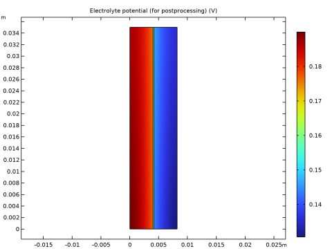
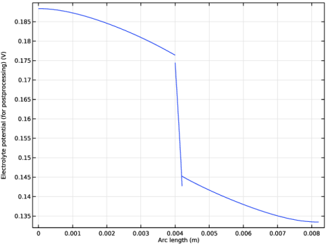
In the Settings window for Line Graph, click Replace Expression in the upper-right corner of the y-Axis Data section. From the menu, choose Component 1 (comp1) > Definitions > Variables > phil - Electrolyte potential (for postprocessing) - V.
3
In the 1D Plot Group 4 toolbar, click  Plot.
Electrolyte potential
1
In the Model Builder window, right-click 1D Plot Group 4 and choose Rename.
2
In the Rename 1D Plot Group dialog, type Electrolyte potential in the New label text field.
3
1D Plot Group 5
1
In the Results toolbar, click  1D Plot Group.
2
In the Settings window for 1D Plot Group, locate the Title section.
3
From the Title type list, choose None.
Line Graph 1
1
Right-click 1D Plot Group 5 and choose Line Graph.
2
In the Settings window for Line Graph, locate the Data section.
3
From the Dataset list, choose Cut Line 2D 1.
4
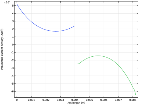
Click Replace Expression in the upper-right corner of the y-Axis Data section. From the menu, choose Component 1 (comp1) > Tertiary Current Distribution, Nernst-Planck (Negative) > Electrode kinetics > tcd.ivtot - Volumetric current density - A/m³.
5
In the 1D Plot Group 5 toolbar, click  Plot.
Line Graph 2
1
Right-click Line Graph 1 and choose Duplicate.
2
In the Settings window for Line Graph, locate the y-Axis Data section.
3
In the Expression text field, type tcd3.ivtot.
4
In the 1D Plot Group 5 toolbar, click  Plot.
Electrode reaction current densities
1
In the Model Builder window, right-click 1D Plot Group 5 and choose Rename.
2
In the Rename 1D Plot Group dialog, type Electrode reaction current densities in the New label text field.
3
2D Plot Group 6
In the Results toolbar, click  2D Plot Group.
Surface 1
1
Right-click 2D Plot Group 6 and choose Surface.
2
In the Settings window for Surface, locate the Expression section.
3
In the Expression text field, type log(abs(rd)).
4
In the 2D Plot Group 6 toolbar, click  Plot.
Dissociation rate
1
In the Model Builder window, right-click 2D Plot Group 6 and choose Rename.
2
In the Rename 2D Plot Group dialog, type Dissociation rate in the New label text field.
3
1D Plot Group 7
1
In the Results toolbar, click  1D Plot Group.
2
In the Settings window for 1D Plot Group, locate the Data section.
3
From the Dataset list, choose Cut Line 2D 1.
4
Locate the Title section. From the Title type list, choose None.
5
Locate the Plot Settings section.
6
Select the y-axis label checkbox. In the associated text field, type Species activity (-).
7
Locate the Legend section. From the Position list, choose Middle right.
Line Graph 1
1
In the Model Builder window, expand the 1D Plot Group 7 node.
2
Right-click 1D Plot Group 7 and choose Line Graph.
3
In the Settings window for Line Graph, locate the y-Axis Data section.
4
In the Expression text field, type aH.
5
Click to expand the Legends section. Select the Show legends checkbox.
6
From the Legends list, choose Manual.
7
Line Graph 2
1
Right-click Line Graph 1 and choose Duplicate.
2
In the Settings window for Line Graph, locate the y-Axis Data section.
3
In the Expression text field, type aHSO4.
4
Locate the Legends section. In the table, enter the following settings:
Line Graph 3
1
Right-click Line Graph 2 and choose Duplicate.
2
In the Settings window for Line Graph, locate the y-Axis Data section.
3
In the Expression text field, type aSO4.
4
Locate the Legends section. In the table, enter the following settings:
Sulfuric acid species
1
In the Model Builder window, click 1D Plot Group 7.
2
In the 1D Plot Group 7 toolbar, click  Plot.
3
In the Settings window for 1D Plot Group, type Sulfuric acid species in the Label text field.
1D Plot Group 8
1
In the Results toolbar, click  1D Plot Group.
2
In the Settings window for 1D Plot Group, locate the Data section.
3
From the Dataset list, choose Cut Line 2D 1.
4
Locate the Title section. From the Title type list, choose None.
5
Locate the Plot Settings section.
6
Select the y-axis label checkbox. In the associated text field, type Species activity (-).
7
Locate the Legend section. From the Position list, choose Middle right.
Line Graph 1
1
Right-click 1D Plot Group 8 and choose Line Graph.
2
In the Settings window for Line Graph, locate the y-Axis Data section.
3
In the Expression text field, type aV2.
4
Locate the Legends section. Select the Show legends checkbox.
5
From the Legends list, choose Manual.
6
Line Graph 2
1
Right-click Line Graph 1 and choose Duplicate.
2
In the Settings window for Line Graph, locate the y-Axis Data section.
3
In the Expression text field, type aV3.
4
Locate the Legends section. In the table, enter the following settings:
Line Graph 3
1
Right-click Line Graph 2 and choose Duplicate.
2
In the Settings window for Line Graph, locate the y-Axis Data section.
3
In the Expression text field, type aV4.
4
Locate the Legends section. In the table, enter the following settings:
Line Graph 4
1
Right-click Line Graph 3 and choose Duplicate.
2
In the Settings window for Line Graph, locate the y-Axis Data section.
3
In the Expression text field, type aV5.
4
Locate the Legends section. In the table, enter the following settings:
V2/V3/V4/V5
1
In the Model Builder window, click 1D Plot Group 8.
2
In the 1D Plot Group 8 toolbar, click  Plot.
3
In the Settings window for 1D Plot Group, type V2/V3/V4/V5 in the Label text field.
1D Plot Group 9
1
In the Results toolbar, click  1D Plot Group.
2
In the Settings window for 1D Plot Group, locate the Data section.
3
From the Dataset list, choose Cut Line 2D 1.
4
Locate the Title section. From the Title type list, choose None.
5
Locate the Plot Settings section.
6
Select the y-axis label checkbox. In the associated text field, type Flux (A/m<sup>2</sup>).
Line Graph 1
1
Right-click 1D Plot Group 9 and choose Line Graph.
2
In the Settings window for Line Graph, locate the y-Axis Data section.
3
In the Expression text field, type Hx*F_const.
4
Locate the Legends section. Select the Show legends checkbox.
5
From the Legends list, choose Manual.
6
Line Graph 2
1
Right-click Line Graph 1 and choose Duplicate.
2
In the Settings window for Line Graph, locate the y-Axis Data section.
3
In the Expression text field, type -HSO4x*F_const.
4
Locate the Legends section. In the table, enter the following settings:
Line Graph 3
1
Right-click Line Graph 2 and choose Duplicate.
2
In the Settings window for Line Graph, locate the y-Axis Data section.
3
In the Expression text field, type -2*F_const*SO4x.
4
Locate the Legends section. In the table, enter the following settings:
Fluxes
1
In the Model Builder window, click 1D Plot Group 9.
2
In the 1D Plot Group 9 toolbar, click  Plot.
3
In the Settings window for 1D Plot Group, type Fluxes in the Label text field.