PDF

Liquid-Cooled Prismatic Battery Pack
Introduction
This tutorial models the temperature profile in a liquid-cooled prismatic battery pack during a high-rate charge.
The pack consists of 16 prismatic battery cells connected by busbars, placed on an aluminum plate containing four cooling channels. The battery pack is assumed to have two faulty cells, featuring higher ohmic resistance values in comparison to the remaining cells in the pack. All other battery cell properties are identical.
The Battery Pack interface using the Two electrodes model is used to set up the current conduction and cell chemistry in the jelly roll, current conductors and busbars. The heat transfer in the battery cells, busbars and cooling plate is modeled using the Heat Transfer in Solids interface, whereas the Heat Transfer in Pipes and the Pipe Flow interface are used to define the convective heat transfer in the cooling channels.
The single battery cell geometry and parameters are similar to that used in the Application Libraries example Cooling of a Prismatic Battery.
Note: This model requires a Pipe Flow Module license.
Model Definition
Figure 1: Prismatic battery pack model geometry.
Figure 1 shows the model geometry. The prismatic battery pack consists of 16 prismatic battery cells connected by busbars. The battery pack is placed on a cooling plate with channels. The channels are defined as 1D edges.
The individual geometry parts that are used to build the battery pack geometry are shown in Figure 2 through Figure 4:
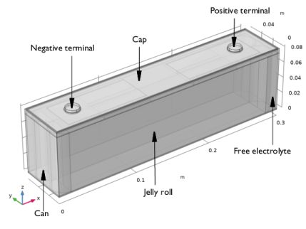
Figure 2 shows a single prismatic battery cell consisting of two jelly rolls. The different components of the single prismatic battery cell are discussed in detail in the Application Libraries example Cooling of a Prismatic Battery.
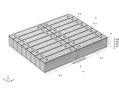
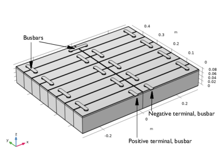
Figure 3 shows 16 prismatic battery cells connected by busbars.
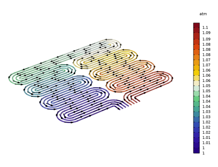
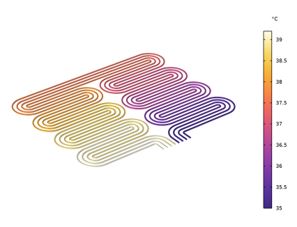
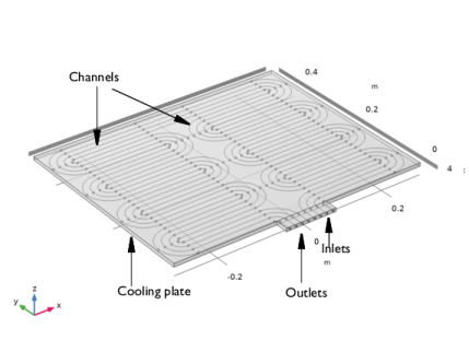
Figure 4 shows the cooling plate with channels.
Figure 2: Single prismatic battery cell.
Figure 3: 16 prismatic battery cells connected by busbars.
Figure 4: Cooling plate with 1D channels.
The following domains and corresponding materials (taken from the Built-in material library, when available) are defined in the model geometry:
Busbars (Copper)
Cell can (Aluminum)
Cap (Aluminum)
Spacer (Acrylic plastic)
Seal (Acrylic plastic)
Battery cell terminals (Copper/Aluminum)
Free electrolyte (user-defined Electrolyte material)
Metal foils (homogenized mixture of Copper/Aluminum and Electrolyte)
Electrochemical Model
The Battery Pack interface with the Two electrodes model is used to set up the physics in the jelly roll (active layers of the battery cell), current conductors (current collectors plates, foils and terminals of the battery cell), and busbars of the prismatic battery pack.
In the model, the battery pack is assumed to have two faulty cells, that have a higher value of ohmic resistance when compared to the remaining cells in the pack. By enabling Specify battery properties from materials on the Batteries node, some model parameters (such as the initial positive and negative host capacities, and overpotential related properties on the Voltage Losses subnode) are defined using nodes defined under the Materials node in the model tree. By the usage of multiple material nodes, it is possible to assign different properties to individual battery cells. The higher ohmic resistance of the two faulty cells in the model are defined using a second material node.
The Specify battery properties from materials checkbox does not control any of the inputs belonging to the Batteries > Negative Equilibrium Potential and Batteries > Positive Equilibrium Potential subnodes. Instead, the negative and positive electrode materials are specified explicitly on these individual subnodes. The half-cell equilibrium potential curves for the two electrode materials, representing graphite and LiFePO4 (LFP) and identical for all cells in the pack, are taken from the Battery material library.
All cells in the pack are set to an initial cell state of charge (SOC) of 10%. A Ground condition is used at the negative terminal busbar boundary, and a Current condition corresponding to 4C cell current is defined on the positive terminal busbar boundary.
The negative and positive connectors, interconnecting the battery cell models and the current conduction domains, are set to the boundaries between the jelly roll and negative and positive foil domains, respectively.
Flow Model
The flow in the channels is described using the Pipe Flow interface. The inlet liquid mass flow rate is set to 0.01 kg/s using the Mass flow rate option.
Heat Transfer Model
The heat transfer in the channels is modeled using Heat Transfer in Pipes interface. For faster computation times, the discretization of the temperature dependent variable is set to linear.
The inlet and initial temperature of the liquid is set to 35°C. The Wall Heat Transfer node is used to set up heat exchange across the pipe wall. The external temperature is set up automatically by the use of Pipe Wall Heat Transfer multiphysics node. An Internal Film Resistance subnode is added, to define the nature of heat transfer and compute the heat transfer coefficient.
Heat Transfer in Solids interface is used to model the temperature distribution in all domains of the battery pack. For faster computation times, the discretization for temperature is set to linear. The heat source from the Battery Pack interface is added by the use of Electrochemical Heating multiphysics node.
The metal foils bundles are treated as homogenized domains and defined using the Porous Medium node, where the thermal properties in the metal/electrolyte mix is defined by the use of Porous Material material nodes. The anisotropic thermal conductivity in the jelly roll is handled using Battery Layers node, where the in-layer and through-layer thermal conductivities are specified. Convective cooling conditions are added by the use of a Heat Flux node on all the top boundaries. The initial temperature of the entire battery pack is set to 35°C.
Study
The model is solved in two steps (a Stationary study step followed by a Time Dependent study step). The steady state fluid flow in the channels is solved for in the Stationary step, at the initial temperature of 35°C. The electrochemical and heat transfer model is solved for in the Time Dependent step. The final pack SOC of 80% is implicitly defined by end time in the Time Dependent step.
Results and Discussion
Figure 5 shows the average, maximum, and minimum battery cell voltages versus time. The temperature variation in the battery pack leads to a variation in the voltage profile across different cells in the battery pack. The cells with higher temperatures will have voltage profiles closer to the maximum cell voltage profile.
Figure 5: Battery cell voltages (average, maximum, and minimum) versus time.
Figure 6 shows the electric potential in the current conductors and busbars. The negative terminal busbar boundary has been grounded.
Figure 6: Electric potential in the current conductors and busbars.
Figure 7 shows the pressure distribution in the channels. The arrows represent the velocity field. Figure 8 shows the temperature distribution (at the end of the simulation) in the channels. The inlet temperature of the liquid in the channels is 35°C. The liquid outlet temperature is about 4°C higher than the liquid inlet temperature.
Figure 7: Pressure distribution in the channels. The arrows represent the velocity field.
Figure 8: Temperature distribution in the channels.
Figure 9: Temperature distribution in the entire battery pack.
Figure 10: Temperature distribution in the jelly roll, current conductors, and busbars.
Figure 9 shows the temperature distribution (at the end of the simulation) in the entire battery pack. There is a variation of about 10°C in the battery pack. The two faulty cells that have a higher value of ohmic resistance than the remaining cells in the battery pack show increased heating and higher temperatures when compared to the adjacent cells in the pack.
Figure 10 shows the temperature distribution (at the end of the simulation) in the jelly roll, current conductors, and busbars. It is evident that the two faulty cells, their current conductors, and the busbars show increased heating and higher temperatures when compared to the adjacent cells in the pack.
Figure 11: Temperature distribution in the cooling plate.
Figure 11 shows the temperature distribution (at the end of the simulation) in the cooling plate. The temperature distribution in the cooling plate is similar to that in the channels, with a variation of about 5°C across the cooling plate. Also, the cooling plate shows increased heating and higher temperatures near the faulty cells.
Application Library path: Battery_Design_Module/Thermal_Management/prismatic_battery_pack_cooling
Modeling Instructions
From the File menu, choose New.
New
In the New window, click  Model Wizard.
Model Wizard
1
In the Model Wizard window, click  3D.
2
In the Select Physics tree, select Electrochemistry > Batteries > Battery Pack (bp).
3
Click Add.
4
In the Select Physics tree, select Fluid Flow > Single-Phase Flow > Pipe Flow (pfl).
5
Click Add.
6
In the Select Physics tree, select Heat Transfer > Heat Transfer in Pipes (htp).
7
Click Add.
8
In the Select Physics tree, select Heat Transfer > Heat Transfer in Solids (ht).
9
Click Add.
10
Click  Study.
11
In the Select Study tree, select Empty Study.
12
Geometry: Battery Pack
Load the geometry sequence from a file as follows:
1
In the Geometry toolbar, click Insert Sequence and choose Insert Sequence.
2
3
In the Insert Sequence dialog, click OK.
4
In the Model Builder window, under Component 1 (comp1) click Geometry 1.
5
In the Settings window for Geometry, type Geometry: Battery Pack in the Label text field.
6
In the Geometry toolbar, click  Build All.
7
Click the  Transparency button in the Graphics toolbar.
8
Click the  Zoom Extents button in the Graphics toolbar.
The prismatic battery pack consists of 16 prismatic battery cells connected by busbars, placed on a cooling plate with four channels. The channels are modeled as edges.
9
Locate the Cleanup section. Clear the Automatic detection of small details checkbox.
10
In the Model Builder window, collapse the Geometry: Battery Pack node.
Global Definitions
Geometry Parameters
Some parameters were imported with the geometry sequence.
1
In the Model Builder window, under Global Definitions click Parameters 1.
2
In the Settings window for Parameters, type Geometry Parameters in the Label text field.
Physics Parameters
Add additional parameters for setting up the physics as follows:
1
In the Home toolbar, click  Parameters and choose Add > Parameters.
2
In the Settings window for Parameters, type Physics Parameters in the Label text field.
3
Locate the Parameters section. Click  Load from File.
4
5
Click  Load from File.
6
Browse to the model’s Application Libraries folder and double-click the file prismatic_battery_pack_cooling_physics_parameters.txt.
Add Material
Add data for the graphite and LFP electrode from the Battery material library, as Global materials. Additional materials which will be assigned to different domains of the prismatic battery pack, will be added later.
1
In the Materials toolbar, click  Add Material to open the Add Material window.
2
Go to the Add Material window.
3
In the tree, select Battery > Electrodes > Graphite, LixC6 MCMB (Negative, Li-ion Battery).
4
Right-click and choose Add to Global Materials.
5
In the tree, select Battery > Electrodes > LFP, LiFePO4 (Positive, Li-ion Battery).
6
Right-click and choose Add to Global Materials.
7
In the Materials toolbar, click  Add Material to close the Add Material window.
Definitions
Variables 1
Add some variables as follows:
1
In the Model Builder window, under Component 1 (comp1) right-click Definitions and choose Variables.
2
In the Settings window for Variables, locate the Variables section.
3
Click  Load from File.
4
Browse to the model’s Application Libraries folder and double-click the file prismatic_battery_pack_cooling_physics_variables.txt.
Multiphysics
Before we set up the physics, add the required Multiphysics coupling nodes.
Pipe Wall Heat Transfer 1 (pwhtc1)
In the Physics toolbar, click  Multiphysics Couplings and choose Edge > Pipe Wall Heat Transfer.
Electrochemical Heating 1 (ech1)
In the Physics toolbar, click  Multiphysics Couplings and choose Domain > Electrochemical Heating.
Battery Pack (bp)
Start setting up the physics, starting with the electrochemical model. The Battery Pack interface using the Two electrodes model is used to set up the physics in the jelly roll, current conductors and busbars.
1
In the Model Builder window, under Component 1 (comp1) click Battery Pack (bp).
2
In the Settings window for Battery Pack, locate the Domain Selection section.
3
From the Selection list, choose Jelly Roll, Current Conductors and Busbars (Batteries and Busbars).
Batteries
1
In the Model Builder window, under Component 1 (comp1) > Battery Pack (bp) click Batteries.
2
In the Settings window for Batteries, locate the Domain Selection section.
3
From the Selection list, choose Jelly Roll (Battery Cell 1) (Batteries and Busbars).
4
Locate the Battery Pack Settings section. From the Model list, choose Two electrodes.
5
Select the Specify battery properties from materials checkbox.
The checkbox Specify battery properties from materials allows to automatically set up some inputs from a material specified in the Materials node, that has been assigned to the selection of the Batteries node. This jelly roll material will be added later in the Materials node.
6
Locate the Initial Cell Charge Distribution section. In the SOCcell,0 text field, type SOC_init.
Negative Equilibrium Potential 1
Specify the negative electrode material explicitly as follows:
1
In the Model Builder window, click Negative Equilibrium Potential 1.
2
In the Settings window for Negative Equilibrium Potential, locate the Material section.
3
From the Electrode material list, choose Graphite, LixC6 MCMB (Negative, Li-ion Battery) (mat1).
Positive Equilibrium Potential 1
Similarly, specify the positive electrode material explicitly.
1
In the Model Builder window, click Positive Equilibrium Potential 1.
2
In the Settings window for Positive Equilibrium Potential, locate the Material section.
3
From the Electrode material list, choose LFP, LiFePO4 (Positive, Li-ion Battery) (mat2).
Voltage Losses 1
1
In the Model Builder window, click Voltage Losses 1.
2
In the Settings window for Voltage Losses, locate the Concentration Overpotential, Negative section.
3
Select the Include concentration overpotential, negative checkbox.
4
Locate the Concentration Overpotential, Positive section. Select the Include concentration overpotential, positive checkbox.
Current Conductors
1
In the Model Builder window, under Component 1 (comp1) > Battery Pack (bp) click Current Conductors.
2
In the Settings window for Current Conductors, locate the Domain Selection section.
3
From the Selection list, choose Current Conductors and Busbars (Batteries and Busbars).
Ground 1
1
In the Physics toolbar, click  Attributes and choose Ground.
2
In the Settings window for Ground, locate the Boundary Selection section.
3
From the Selection list, choose Busbar Boundary, Negative Terminal (Batteries and Busbars).
Current Conductors
In the Model Builder window, click Current Conductors.
Current 1
1
In the Physics toolbar, click  Attributes and choose Current.
2
In the Settings window for Current, locate the Boundary Selection section.
3
From the Selection list, choose Busbar Boundary, Positive Terminal (Batteries and Busbars).
4
Locate the Electrode Current section. In the Is,total text field, type I_app.
Negative Connectors
1
In the Model Builder window, under Component 1 (comp1) > Battery Pack (bp) click Negative Connectors.
2
In the Settings window for Negative Connectors, locate the Boundary Selection section.
3
From the Selection list, choose Negative Foils - Jelly Roll Boundaries (Battery Cell 1) (Batteries and Busbars).
Positive Connectors
1
In the Model Builder window, click Positive Connectors.
2
In the Settings window for Positive Connectors, locate the Boundary Selection section.
3
From the Selection list, choose Positive Foils - Jelly Roll Boundaries (Battery Cell 1) (Batteries and Busbars).
Pipe Flow (pfl)
Next set up the physics for flow in the channels using the Pipe Flow interface. Again, the fluid material will be added later in the Materials node.
1
In the Model Builder window, under Component 1 (comp1) click Pipe Flow (pfl).
2
In the Settings window for Pipe Flow, locate the Edge Selection section.
3
From the Selection list, choose Channels (Cooling Plate and Channels).
Pipe Properties 1
1
In the Model Builder window, under Component 1 (comp1) > Pipe Flow (pfl) click Pipe Properties 1.
2
In the Settings window for Pipe Properties, locate the Pipe Shape section.
3
4
In the wi text field, type s_channels.
Inlet 1
1
In the Physics toolbar, click  Points and choose Inlet.
2
In the Settings window for Inlet, locate the Point Selection section.
3
From the Selection list, choose Inlets (Cooling Plate and Channels).
4
Locate the Inlet Specification section. In the qm,0 text field, type M_flow_in.
Heat Transfer in Pipes (htp)
Next set up the physics for heat transfer in the channels using the Heat Transfer in Pipes interface. For faster computation times, the Discretization for temperature is set to Linear.
1
In the Model Builder window, under Component 1 (comp1) click Heat Transfer in Pipes (htp).
2
In the Settings window for Heat Transfer in Pipes, locate the Edge Selection section.
3
From the Selection list, choose Channels (Cooling Plate and Channels).
4
Click to expand the Discretization section. From the Temperature list, choose Linear.
Heat Transfer 1
1
In the Model Builder window, under Component 1 (comp1) > Heat Transfer in Pipes (htp) click Heat Transfer 1.
2
In the Settings window for Heat Transfer, locate the Heat Convection and Conduction section.
3
From the u list, choose Tangential velocity (pfl).
Pipe Properties 1
1
In the Model Builder window, click Pipe Properties 1.
2
In the Settings window for Pipe Properties, locate the Pipe Shape section.
3
4
In the wi text field, type s_channels.
Temperature 1
1
In the Model Builder window, click Temperature 1.
2
In the Settings window for Temperature, locate the Temperature section.
3
In the Tin text field, type T0.
Initial Values 1
1
In the Model Builder window, click Initial Values 1.
2
In the Settings window for Initial Values, locate the Initial Values section.
3
In the T text field, type T0.
Heat Outflow 1
1
In the Physics toolbar, click  Points and choose Heat Outflow.
2
In the Settings window for Heat Outflow, locate the Point Selection section.
3
From the Selection list, choose Outlets (Cooling Plate and Channels).
Wall Heat Transfer 1
The Wall Heat Transfer node is used to set up heat exchange across the pipe wall. The external temperature is set up automatically from the Pipe Wall Heat Transfer multiphysics node. An Internal Film Resistance subnode is added, to define the nature of heat transfer and compute the heat transfer coefficient.
1
In the Physics toolbar, click  Edges and choose Wall Heat Transfer.
2
In the Settings window for Wall Heat Transfer, locate the Edge Selection section.
3
From the Selection list, choose Channels (Cooling Plate and Channels).
Internal Film Resistance 1
In the Physics toolbar, click  Attributes and choose Internal Film Resistance.
Heat Transfer in Solids (ht)
Finally set up the physics for heat transfer in all domains using the Heat Transfer in solids interface. For faster computation times, the Discretization for temperature is set to Linear. The heat source from the Battery Pack interface is added from the Electrochemical Heating multiphysics node. Again, all required materials will be added later in the Materials node.
1
In the Model Builder window, under Component 1 (comp1) click Heat Transfer in Solids (ht).
2
In the Settings window for Heat Transfer in Solids, click to expand the Discretization section.
3
From the Temperature list, choose Linear.
Initial Values 1
1
In the Model Builder window, under Component 1 (comp1) > Heat Transfer in Solids (ht) click Initial Values 1.
2
In the Settings window for Initial Values, locate the Initial Values section.
3
In the T2 text field, type T0.
Porous Medium 1
The foil domains are modeled as porous media, consisting of a mix of metal conductors and electrolyte.
1
In the Physics toolbar, click  Domains and choose Porous Medium.
2
In the Settings window for Porous Medium, locate the Domain Selection section.
3
From the Selection list, choose Foils (Battery Cell 1) (Batteries and Busbars).
Battery Layers 1
Define the heat transfer within the jelly roll as follows:
1
In the Physics toolbar, click  Domains and choose Battery Layers.
2
In the Settings window for Battery Layers, locate the Domain Selection section.
3
From the Selection list, choose Jelly Roll (Battery Cell 1) (Batteries and Busbars).
4
Locate the Battery Layers section. From the Layer configuration list, choose Flat-sided oval (prismatic).
5
In the ktl text field, type kT_batt_tl.
6
In the kil text field, type kT_batt_il.
7
In the ρeff text field, type rho_batt.
8
In the Cp,eff text field, type Cp_batt.
Rectangular Block Selection 1
1
In the Model Builder window, click Rectangular Block Selection 1.
2
In the Settings window for Rectangular Block Selection, locate the Domain Selection section.
3
From the Selection list, choose Jelly Roll Rectangular Blocks (Battery Cell 1) (Batteries and Busbars).
4
Locate the Battery Layers section. From the Through-layer direction list, choose y-axis.
Heat Flux 1
1
In the Physics toolbar, click  Boundaries and choose Heat Flux.
2
In the Settings window for Heat Flux, locate the Boundary Selection section.
3
From the Selection list, choose Pack Convective Boundaries (Batteries and Busbars).
4
Locate the Heat Flux section. From the Flux type list, choose Convective heat flux.
5
In the h text field, type htc.
6
In the Text text field, type T0.
Materials
Add all the materials required by the physics interfaces and assign them to appropriate domains or edges.
Add Material from Library
In the Home toolbar, click  Windows and choose Add Material from Library.
Add Material
1
Go to the Add Material window.
2
In the tree, select Liquids and Gases > Liquids > Water.
3
Click the Add to Component button in the window toolbar.
Materials
Water (mat3)
1
In the Settings window for Material, locate the Geometric Entity Selection section.
2
From the Geometric entity level list, choose Edge.
3
From the Selection list, choose Channels (Cooling Plate and Channels).
Add Material
1
Go to the Add Material window.
2
In the tree, select Built-in > Aluminum.
3
Click the Add to Component button in the window toolbar.
Materials
Aluminum (mat4)
1
In the Settings window for Material, locate the Geometric Entity Selection section.
2
From the Selection list, choose Pack Aluminum Domains.
Add Material
1
Go to the Add Material window.
2
In the tree, select Built-in > Copper.
3
Click the Add to Component button in the window toolbar.
Materials
Copper (mat5)
1
In the Settings window for Material, locate the Geometric Entity Selection section.
2
From the Selection list, choose Pack Copper Domains.
Add Material
1
Go to the Add Material window.
2
In the tree, select Built-in > Acrylic plastic.
3
Click the Add to Component button in the window toolbar.
4
In the Home toolbar, click  Add Material to close the Add Material window.
Materials
Acrylic plastic (mat6)
1
In the Settings window for Material, locate the Geometric Entity Selection section.
2
From the Selection list, choose Spacer and Seal (Battery Cell 1) (Batteries and Busbars).
Electrolyte
1
In the Model Builder window, right-click Materials and choose Blank Material.
2
In the Settings window for Material, type Electrolyte in the Label text field.
3
Locate the Geometric Entity Selection section. From the Selection list, choose Free Electrolyte (Battery Cell 1) (Batteries and Busbars).
4
Locate the Material Contents section. In the table, enter the following settings:
Porous Material - Homogenized Negative Foils
1
Right-click Materials and choose More Materials > Porous Material.
2
In the Settings window for Porous Material, type Porous Material - Homogenized Negative Foils in the Label text field.
3
Locate the Geometric Entity Selection section. From the Selection list, choose Negative Foils (Battery Cell 1) (Batteries and Busbars).
Fluid 1 (pmat1.fluid1)
1
Right-click Porous Material - Homogenized Negative Foils and choose Fluid.
2
In the Settings window for Fluid, locate the Fluid Properties section.
3
From the Material list, choose Electrolyte (mat7).
Solid 1 (pmat1.solid1)
1
In the Model Builder window, right-click Porous Material - Homogenized Negative Foils (pmat1) and choose Solid.
2
In the Settings window for Solid, locate the Solid Properties section.
3
From the Material list, choose Copper (mat5).
4
In the θs text field, type eps_cc_neg.
Porous Material - Homogenized Negative Foils (pmat1)
1
In the Model Builder window, click Porous Material - Homogenized Negative Foils (pmat1).
2
In the Settings window for Porous Material, locate the Homogenized Properties section.
3
Porous Material - Homogenized Positive Foils
1
In the Model Builder window, right-click Materials and choose More Materials > Porous Material.
2
In the Settings window for Porous Material, type Porous Material - Homogenized Positive Foils in the Label text field.
3
Locate the Geometric Entity Selection section. From the Selection list, choose Positive Foils (Battery Cell 1) (Batteries and Busbars).
Fluid 1 (pmat2.fluid1)
1
Right-click Porous Material - Homogenized Positive Foils and choose Fluid.
2
In the Settings window for Fluid, locate the Fluid Properties section.
3
From the Material list, choose Electrolyte (mat7).
Solid 1 (pmat2.solid1)
1
In the Model Builder window, right-click Porous Material - Homogenized Positive Foils (pmat2) and choose Solid.
2
In the Settings window for Solid, locate the Solid Properties section.
3
From the Material list, choose Aluminum (mat4).
4
In the θs text field, type eps_cc_pos.
Porous Material - Homogenized Positive Foils (pmat2)
1
In the Model Builder window, click Porous Material - Homogenized Positive Foils (pmat2).
2
In the Settings window for Porous Material, locate the Homogenized Properties section.
3
Jelly Roll Material
In this model, the battery pack is assumed to have two faulty cells, featuring higher ohmic resistance values in comparison to the remaining cells in the pack. All other battery cell properties are identical. Set up the jelly roll materials as follows:
1
In the Model Builder window, right-click Materials and choose Blank Material.
2
In the Settings window for Material, type Jelly Roll Material in the Label text field.
3
Locate the Geometric Entity Selection section. From the Selection list, choose Jelly Roll (Battery Cell 1) (Batteries and Busbars).
4
Locate the Material Contents section. In the table, enter the following settings:
Jelly Roll Material, Faulty
1
Right-click Jelly Roll Material and choose Duplicate.
2
In the Settings window for Material, type Jelly Roll Material, Faulty in the Label text field.
3
Locate the Geometric Entity Selection section. From the Selection list, choose Faulty Jelly Roll.
4
Locate the Material Contents section. In the table, enter the following settings:
Pipe Flow (pfl)
Fluid Properties 1
Set the model input temperature in the Pipe Flow interface to be the initial temperature. The steady state fluid flow in the channels will be solved for in a Stationary study step only.
1
In the Model Builder window, under Component 1 (comp1) > Pipe Flow (pfl) click Fluid Properties 1.
2
In the Settings window for Fluid Properties, locate the Model Input section.
3
In the T text field, type T0.
Definitions (comp1)
Set up some probes for the cell voltage as follows:
Global Variable Probe: E_cell average
1
In the Definitions toolbar, click  Probes and choose Global Variable Probe.
2
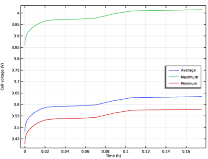
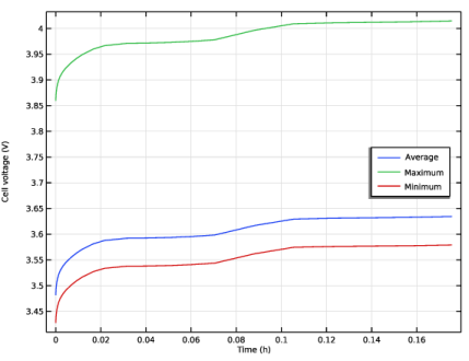
In the Settings window for Global Variable Probe, type Global Variable Probe: E_cell average in the Label text field.
3
Locate the Expression section. In the Expression text field, type bp.E_cell_avg.
4
Select the Description checkbox. In the associated text field, type Cell voltage, average.
Global Variable Probe: E_cell maximum
1
Right-click Global Variable Probe: E_cell average and choose Duplicate.
2
In the Settings window for Global Variable Probe, type Global Variable Probe: E_cell maximum in the Label text field.
3
Locate the Expression section. In the Expression text field, type bp.E_cell_max.
4
In the Description text field, type Cell voltage, maximum.
Global Variable Probe: E_cell minimum
1
Right-click Global Variable Probe: E_cell maximum and choose Duplicate.
2
In the Settings window for Global Variable Probe, type Global Variable Probe: E_cell minimum in the Label text field.
3
Locate the Expression section. In the Expression text field, type bp.E_cell_min.
4
In the Description text field, type Cell voltage, minimum.
Mesh 1
Set up a user-defined mesh as follows:
1
In the Model Builder window, under Component 1 (comp1) click Mesh 1.
2
In the Settings window for Mesh, locate the Sequence Type section.
3
From the list, choose User-controlled mesh.
4
In the Mesh toolbar, click  Clear Sequence.
Free Tetrahedral 1
1
In the Mesh toolbar, click  Free Tetrahedral.
2
In the Settings window for Free Tetrahedral, locate the Domain Selection section.
3
From the Geometric entity level list, choose Domain.
4
From the Selection list, choose Cooling Plate (Cooling Plate and Channels).
Size 1
1
Right-click Free Tetrahedral 1 and choose Size.
2
In the Settings window for Size, locate the Geometric Entity Selection section.
3
From the Geometric entity level list, choose Edge.
4
From the Selection list, choose Channels (Cooling Plate and Channels).
5
Locate the Element Size section. Click the Custom button.
6
Locate the Element Size Parameters section.
7
Select the Maximum element size checkbox. In the associated text field, type s_channels.
8
Click  Build Selected.
Free Tetrahedral 2
1
In the Mesh toolbar, click  Free Tetrahedral.
2
In the Settings window for Free Tetrahedral, locate the Domain Selection section.
3
From the Geometric entity level list, choose Domain.
4
From the Selection list, choose Battery Free Tet Domains (Battery Cell 1) (Batteries and Busbars).
Size 1
1
Right-click Free Tetrahedral 2 and choose Size.
2
In the Settings window for Size, locate the Geometric Entity Selection section.
3
From the Geometric entity level list, choose Edge.
4
From the Selection list, choose Jelly Roll Envelope Edges (Battery Cell 1) (Batteries and Busbars).
5
Locate the Element Size section. Click the Custom button.
6
Locate the Element Size Parameters section.
7
Select the Maximum element size checkbox. In the associated text field, type s_can*2.
8
Click  Build Selected.
Swept 1
1
In the Mesh toolbar, click  Swept.
2
In the Settings window for Swept, locate the Domain Selection section.
3
From the Geometric entity level list, choose Domain.
4
From the Selection list, choose Battery Upper Sweep Domains (Battery Cell 1) (Batteries and Busbars).
Size 1
1
Right-click Swept 1 and choose Size.
2
In the Settings window for Size, locate the Element Size section.
3
Click the Custom button.
4
Locate the Element Size Parameters section.
5
Select the Maximum element size checkbox. In the associated text field, type s_can.
6
Click  Build Selected.
Free Tetrahedral 3
1
In the Mesh toolbar, click  Free Tetrahedral.
2
In the Settings window for Free Tetrahedral, locate the Domain Selection section.
3
From the Geometric entity level list, choose Domain.
4
From the Selection list, choose Battery Other Free Tet Domains (Battery Cell 1) (Batteries and Busbars).
5
Click  Build Selected.
Swept 2
1
In the Mesh toolbar, click  Swept.
2
In the Settings window for Swept, locate the Domain Selection section.
3
From the Geometric entity level list, choose Domain.
4
From the Selection list, choose Extrude - Jelly Roll and Can (Battery Cell 1) (Batteries and Busbars).
Distribution 1
1
Right-click Swept 2 and choose Distribution.
2
In the Settings window for Distribution, locate the Domain Selection section.
3
From the Selection list, choose Extrude - Jelly Roll and Can (Battery Cell 1) (Batteries and Busbars).
4
Click  Build Selected.
Free Tetrahedral 4
1
In the Mesh toolbar, click  Free Tetrahedral.
2
In the Settings window for Free Tetrahedral, click  Build Selected.
3
In the Model Builder window, right-click Mesh 1 and choose Build All.
Study 1
The model is now ready for solving. Add a Stationary study step followed by a Time Dependent study step. The Pipe Flow interface (fluid flow in the channels) will be solved for in the Stationary study step only.
Step 1: Stationary
1
In the Study toolbar, click  Stationary.
2
In the Settings window for Stationary, locate the Physics and Variables Selection section.
3
In the Solve for column of the table, under Component 1 (comp1), clear the checkboxes for Heat Transfer in Pipes (htp) and Heat Transfer in Solids (ht).
4
In the Solve for column of the table, under Component 1 (comp1) > Multiphysics, clear the checkboxes for Pipe Wall Heat Transfer 1 (pwhtc1) and Electrochemical Heating 1 (ech1).
Step 2: Time Dependent
1
In the Study toolbar, click  Time Dependent.
2
In the Settings window for Time Dependent, locate the Physics and Variables Selection section.
3
In the Solve for column of the table, under Component 1 (comp1), clear the checkbox for Pipe Flow (pfl).
4
Locate the Study Settings section. From the Time unit list, choose h.
5
In the Output times text field, type range(0,0.1/C_rate,SOC_window/C_rate).
6
In the Study toolbar, click  Compute.
Results
Set the Preferred units to be used for temperature in the plots. Some plots are created by default. Analyze them and create a few additional plots as follows:
Preferred Units 1
1
In the Results toolbar, click  Configurations and choose Preferred Units.
2
In the Settings window for Preferred Units, locate the Units section.
3
Click  Add Physical Quantity.
4
In the Physical Quantity dialog, select General > Temperature (K) in the tree.
5
6
In the Settings window for Preferred Units, locate the Units section.
7
Click  Add Physical Quantity.
8
In the Physical Quantity dialog, select General > Pressure (Pa) in the tree.
9
10
In the Settings window for Preferred Units, locate the Units section.
11
12
Click  Apply.
Jelly Roll Voltage Probe
1
In the Model Builder window, under Results click Probe Plot Group 1.
2
In the Settings window for 1D Plot Group, type Jelly Roll Voltage Probe in the Label text field.
3
Locate the Plot Settings section.
4
Select the y-axis label checkbox. In the associated text field, type Cell voltage (V).
5
Locate the Legend section. From the Position list, choose Middle right.
Probe Table Graph 1
1
In the Model Builder window, expand the Jelly Roll Voltage Probe node, then click Probe Table Graph 1.
2
In the Settings window for Table Graph, click to expand the Legends section.
3
From the Legends list, choose Manual.
4
5
In the Jelly Roll Voltage Probe toolbar, click  Plot.
Electric Potential - Current Conductors and Busbars
1
In the Model Builder window, under Results click Electric Potential (bp).
2
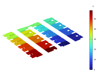
In the Settings window for 3D Plot Group, type Electric Potential - Current Conductors and Busbars in the Label text field.
3
Click to expand the Title section. From the Title type list, choose None.
4
Locate the Plot Settings section. Clear the Plot dataset edges checkbox.
5
Locate the Color Legend section. Select the Show units checkbox.
6
Click the  Transparency button in the Graphics toolbar.
7
Click the  Show Grid button in the Graphics toolbar.
8
Click the  Show Axis Orientation button in the Graphics toolbar.
9
Click the  Zoom Extents button in the Graphics toolbar.
10
In the Electric Potential - Current Conductors and Busbars toolbar, click  Plot.
Pressure - Channels
1
In the Model Builder window, under Results click Pressure (pfl).
2
In the Settings window for 3D Plot Group, type Pressure - Channels in the Label text field.
3
Click to expand the Title section. From the Title type list, choose None.
4
Locate the Plot Settings section. Clear the Plot dataset edges checkbox.
5
Locate the Color Legend section. Select the Show units checkbox.
Transparency 1
1
In the Model Builder window, expand the Pressure - Channels node.
2
Right-click Line 1 and choose Transparency.
Arrow Line 1
1
In the Model Builder window, right-click Pressure - Channels and choose Arrow Line.
2
In the Settings window for Arrow Line, click Replace Expression in the upper-right corner of the Expression section. From the menu, choose Component 1 (comp1) > Pipe Flow > pfl.vX,pfl.vY,pfl.vZ - Velocity.
3
Locate the Coloring and Style section. From the Arrow base list, choose Center.
4
Select the Scale factor checkbox. In the associated text field, type 0.06.
5
From the Color list, choose Black.
Selection 1
1
Right-click Arrow Line 1 and choose Selection.
2
In the Settings window for Selection, locate the Selection section.
3
From the Selection list, choose Channels (Cooling Plate and Channels).
Pressure - Channels
1
Click the  Zoom Extents button in the Graphics toolbar.
2
In the Model Builder window, under Results click Pressure - Channels.
3
In the Pressure - Channels toolbar, click  Plot.
Temperature - Channels
1
In the Model Builder window, under Results click Temperature (htp).
2
In the Settings window for 3D Plot Group, type Temperature - Channels in the Label text field.
3
Locate the Title section. From the Title type list, choose None.
4
Locate the Plot Settings section. Clear the Plot dataset edges checkbox.
5
Locate the Color Legend section. Select the Show units checkbox.
6
Click the  Zoom Extents button in the Graphics toolbar.
7
In the Temperature - Channels toolbar, click  Plot.
Temperature - Full Geometry
1
In the Model Builder window, under Results click Temperature (ht).
2
In the Settings window for 3D Plot Group, type Temperature - Full Geometry in the Label text field.
3
Locate the Title section. From the Title type list, choose None.
4
Locate the Plot Settings section. Clear the Plot dataset edges checkbox.
5
Locate the Color Legend section. Select the Show units checkbox.
6
Click the  Zoom Extents button in the Graphics toolbar.
7
In the Temperature - Full Geometry toolbar, click  Plot.
Temperature - Jelly Roll, Current Conductors and Busbars
1
Right-click Temperature - Full Geometry and choose Duplicate.
2
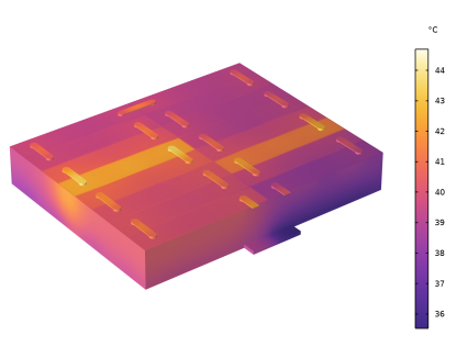
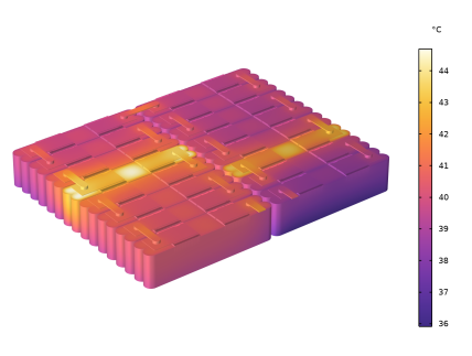
In the Settings window for 3D Plot Group, type Temperature - Jelly Roll, Current Conductors and Busbars in the Label text field.
Selection 1
1
In the Model Builder window, expand the Temperature - Jelly Roll, Current Conductors and Busbars node.
2
Right-click Volume 1 and choose Selection.
3
In the Settings window for Selection, locate the Selection section.
4
From the Selection list, choose Jelly Roll, Current Conductors and Busbars (Batteries and Busbars).
Temperature - Jelly Roll, Current Conductors and Busbars
1
Click the  Zoom Extents button in the Graphics toolbar.
2
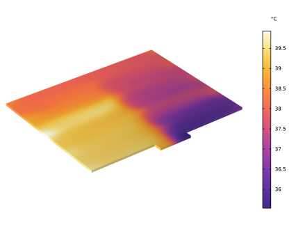
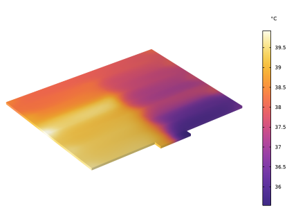
In the Model Builder window, under Results click Temperature - Jelly Roll, Current Conductors and Busbars.
3
In the Temperature - Jelly Roll, Current Conductors and Busbars toolbar, click  Plot.
Temperature - Cooling Plate
1
Right-click Temperature - Jelly Roll, Current Conductors and Busbars and choose Duplicate.
2
In the Settings window for 3D Plot Group, type Temperature - Cooling Plate in the Label text field.
3
In the Model Builder window, expand the Temperature - Cooling Plate node.
Selection 1
1
In the Model Builder window, expand the Results > Temperature - Cooling Plate > Volume 1 node, then click Selection 1.
2
In the Settings window for Selection, locate the Selection section.
3
From the Selection list, choose Cooling Plate (Cooling Plate and Channels).
Temperature - Cooling Plate
1
Click the  Zoom Extents button in the Graphics toolbar.
2
In the Model Builder window, under Results click Temperature - Cooling Plate.
3
In the Temperature - Cooling Plate toolbar, click  Plot.