|
|
|
|
•
|
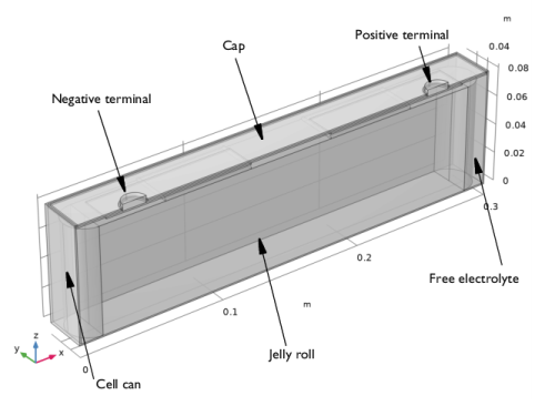
Cell can (Aluminum)
|
|
•
|
Cap (Aluminum)
|
|
•
|
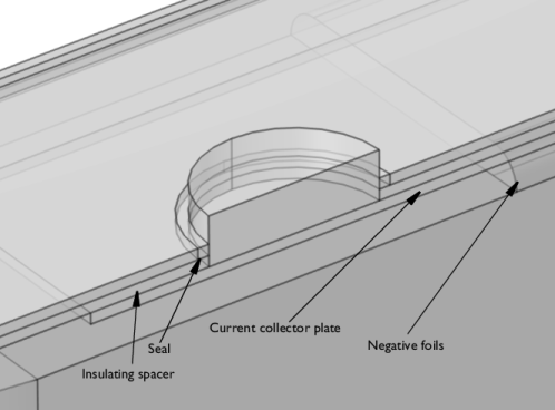
Spacer (Acrylic plastic)
|
|
•
|
Seal (Acrylic plastic)
|
|
•
|
|
•
|
|
•
|
Free electrolyte (user-defined Electrolyte material)
|
|
•
|


|
1
|
|
2
|
In the Select Physics tree, select Electrochemistry > Batteries > Lumped Battery, Two Electrodes (lb).
|
|
3
|
Click Add.
|
|
4
|
Click
|
|
5
|
|
6
|
Click
|
|
1
|
|
2
|
Browse to the model’s Application Libraries folder and double-click the file prismatic_battery_cooling_geom_sequence.mph.
|
|
1
|
|
2
|
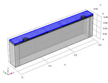
On the object fin, select Boundaries 6, 9, 19, 69, 72, 137, 140, and 157 only.
|
|
1
|
|
2
|
|
3
|
|
4
|
|
1
|
|
2
|
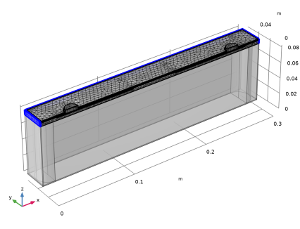
Select the object csol1 only.
|
|
3
|
|
4
|
|
5
|
Click
|
|
1
|
|
2
|
|
3
|
|
4
|
|
5
|
On the object par1, select Domains 1–3, 7–10, 15, 17, 19, 21, 24, 25, 27, 29, 31, 33, 34, 38, 39, 41, 43, 45, and 46 only.
|
|
6
|
|
7
|
|
8
|
|
9
|
|
10
|
Clear the Automatic detection of small details checkbox.
|
|
11
|
|
1
|
|
2
|
|
1
|
|
2
|
|
3
|
|
4
|
Browse to the model’s Application Libraries folder and double-click the file prismatic_battery_cooling_physics_parameters.txt.
|
|
1
|
|
2
|
Go to the Add Material window.
|
|
3
|
|
4
|
Right-click and choose Add to Global Materials.
|
|
5
|
|
6
|
Right-click and choose Add to Global Materials.
|
|
7
|
|
1
|
|
2
|
|
3
|
|
4
|
|
5
|
|
6
|
|
7
|
|
1
|
In the Model Builder window, under Component 1 (comp1) > Lumped Battery (lb) click Negative Equilibrium Potential 1.
|
|
2
|
|
3
|
|
1
|
|
2
|
|
3
|
|
1
|
|
2
|
|
3
|
|
4
|
|
5
|
|
6
|
Locate the Concentration Overpotential, Negative section. Select the Include concentration overpotential, negative checkbox.
|
|
7
|
|
8
|
Locate the Concentration Overpotential, Positive section. Select the Include concentration overpotential, positive checkbox.
|
|
9
|
|
1
|
|
2
|
|
3
|
|
4
|
|
5
|
|
1
|
|
2
|
|
3
|
|
4
|
|
1
|
|
2
|
Go to the Add Physics window.
|
|
3
|
In the tree, select Electrochemistry > Primary and Secondary Current Distribution > Primary Current Distribution (cd).
|
|
4
|
Click the Add to Component 1 button in the window toolbar.
|
|
5
|
|
1
|
|
2
|
|
1
|
|
2
|
|
3
|
|
1
|
|
2
|
|
3
|
|
1
|
|
2
|
|
3
|
|
1
|
|
2
|
|
3
|
|
4
|
|
1
|
|
2
|
|
3
|
|
4
|
|
1
|
|
2
|
Go to the Add Material window.
|
|
3
|
|
4
|
Right-click and choose Add to Component 1 (comp1).
|
|
1
|
|
2
|
|
3
|
|
1
|
Go to the Add Material window.
|
|
2
|
|
3
|
Right-click and choose Add to Component 1 (comp1).
|
|
4
|
|
1
|
|
2
|
|
1
|
In the Model Builder window, under Study 1 right-click Solver Configurations and choose Delete Configurations.
|
|
2
|
|
1
|
|
2
|
Go to the Add Physics window.
|
|
3
|
|
4
|
Click the Add to Component 1 button in the window toolbar.
|
|
5
|
|
1
|
In the Model Builder window, under Component 1 (comp1) > Heat Transfer in Solids (ht) click Initial Values 1.
|
|
2
|
|
3
|
|
1
|
|
2
|
|
3
|
|
1
|
|
2
|
|
3
|
|
4
|
Locate the Battery Layers section. From the Layer configuration list, choose Flat-sided oval (prismatic).
|
|
5
|
|
6
|
|
7
|
|
8
|
|
1
|
|
2
|
|
3
|
|
4
|
|
1
|
|
3
|
|
4
|
|
1
|
|
2
|
|
3
|
|
4
|
|
5
|
|
6
|
|
1
|
|
2
|
Go to the Add Material window.
|
|
3
|
|
4
|
Right-click and choose Add to Component 1 (comp1).
|
|
5
|
|
1
|
|
2
|
|
1
|
|
2
|
|
3
|
|
4
|
Locate the Material Contents section. In the table, enter the following settings:
|
|
1
|
|
2
|
In the Settings window for Porous Material, type Porous Material - Homogenized Negative Foils in the Label text field.
|
|
3
|
|
1
|
|
2
|
|
3
|
|
1
|
In the Model Builder window, right-click Porous Material - Homogenized Negative Foils (pmat1) and choose Solid.
|
|
2
|
|
3
|
|
4
|
|
1
|
|
2
|
|
1
|
|
2
|
In the Settings window for Porous Material, type Porous Material - Homogenized Positive Foils in the Label text field.
|
|
3
|
|
1
|
|
2
|
|
3
|
|
1
|
In the Model Builder window, right-click Porous Material - Homogenized Positive Foils (pmat2) and choose Solid.
|
|
2
|
|
3
|
|
4
|
|
1
|
|
2
|
|
1
|
|
2
|
|
3
|
|
1
|
|
2
|
|
3
|
From the list, choose User-controlled mesh.
|
|
4
|
|
1
|
|
2
|
|
3
|
|
4
|
|
1
|
|
2
|
|
3
|
|
4
|
|
5
|
|
6
|
Locate the Element Size Parameters section.
|
|
7
|
|
1
|
|
2
|
|
3
|
|
4
|
|
1
|
|
2
|
|
3
|
Click the Custom button.
|
|
4
|
Locate the Element Size Parameters section.
|
|
5
|
|
6
|
|
1
|
|
2
|
|
3
|
|
4
|
|
5
|
|
1
|
|
2
|
|
3
|
|
4
|
|
1
|
In the Model Builder window, under Study 1 right-click Solver Configurations and choose Delete Configurations.
|
|
2
|
|
3
|
Clear the Generate default plots checkbox.
|
|
4
|
|
1
|
|
2
|
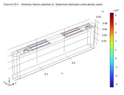
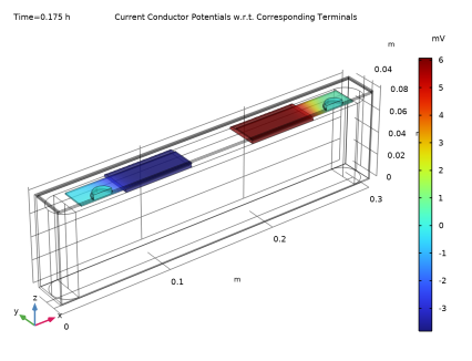
In the Settings window for 3D Plot Group, type Current Conductor Potentials w.r.t. Corresponding Terminals in the Label text field.
|
|
3
|
|
4
|
|
1
|
|
2
|
In the Settings window for Surface, click Replace Expression in the upper-right corner of the Expression section. From the menu, choose Component 1 (comp1) > Primary Current Distribution > cd.phis - Electric potential - V.
|
|
3
|
|
4
|
|
1
|
|
2
|
|
3
|
|
4
|
|
1
|
|
2
|
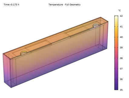
In the Settings window for Volume, click Replace Expression in the upper-right corner of the Expression section. From the menu, choose Component 1 (comp1) > Heat Transfer in Solids > Temperature > T - Temperature - K.
|
|
3
|
|
4
|
|
5
|
|
6
|
|
7
|
|
1
|
|
2
|
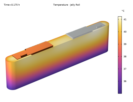
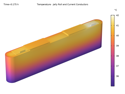
In the Settings window for 3D Plot Group, type Temperature - Jelly Roll and Current Conductors in the Label text field.
|
|
3
|
|
4
|
|
5
|
|
6
|
|
7
|
|
1
|
|
2
|
|
3
|
|
1
|
|
2
|
|
3
|
|
1
|
|
2
|
|
3
|
|
1
|
|
2
|
|
1
|
|
2
|
|
3
|
|
1
|
|
2
|
|
3
|
|
1
|
|
2
|
|
3
|
|
4
|
|
1
|
|
2
|
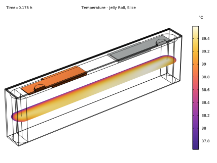
In the Settings window for 3D Plot Group, type Temperature - Jelly Roll, Slice in the Label text field.
|
|
1
|
|
2
|
|
1
|
|
2
|
|
3
|
Select the Plot dataset edges checkbox.
|
|
1
|
|
2
|
|
3
|
|
4
|
|
5
|
|
6
|
|
7
|
|
8
|
|
9
|