PDF

Electrode Utilization in a Large-Format Lithium-Ion Battery Pouch Cell
Introduction
Large lithium-ion batteries are widely employed in electric vehicles and for stationary energy storage applications. In the (stacked) pouch battery cell design, all current exits the cell on the cell “tabs”, and as the cell size and power increases, the voltage gradients in the highly conductive metal foil current collectors may come into play, resulting in a nonuniform current distribution and electrode utilization in the cell. A nonuniform utilization results in suboptimal use of the battery electrodes and may also result in nonuniform and accelerated electrode aging.
This tutorial models the current distribution and electrode utilization in a large format lithium-ion battery pouch cell.
The model is in 3D. Note that all plots are scaled 100 times in the z direction due to the high aspect ratio of the geometric features.
For extended step-by-step instructions for this model, including several screen shots showing how to build it, see the book Introduction to the Battery Design Module.
Model Definition
Figure 1 shows the model geometry. The geometry defines one foil-to-foil unit cell, stacking five layers in the z direction:
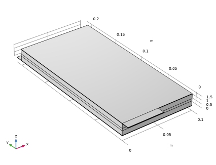
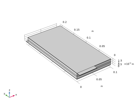
Negative metal current collector foil: 10 μm, Cu (due to symmetry, half of this thickness is used in the model geometry)
Positive metal current collector foil: 10 μm, Al (due to symmetry, half of this thickness is used in the model geometry)
The positive and negative current terminals are located opposite to each other (but may easily be placed on the same side by altering the Geometry node in the model).
Figure 1: Model geometry, scaled 100 times in the z direction.
The Lithium-Ion Battery interface is used to set up the physics, using Material data from the Battery material library.
The Particle Intercalation subnodes to the Porous Electrode nodes model the solid lithium concentration in an additional particle dimension (extra dimension). The model hence defines a fully coupled “pseudo-4D” model.
The SOC and Initial Cell Charge Distribution node is used to set the initial cell state of charge to 20%.
An Electrode Ground boundary condition is used on the negative tab whereas an Electrode Current boundary condition defines the cell current exiting the cell on the positive tab.
A time-dependent solver is use to simulate the charging from a 20% to 90% cell state of charge at a rate of 4C. (A 1C rate corresponds to the charge or discharge current required to fully charge or discharge the battery in 1 h).
Results and Discussion
Figure 2 shows the voltage vs time during the 4C charging period.
Figure 2: Cell voltage versus time.
Figure 3 and Figure 4 show the potential distribution in the negative and positive metal foils (current collector and tab), respectively, at the end of the 4C charge. The potential variation is about 5 mV in the negative current collector and 9 mV in the positive current collector at a 4C charge current.
For a 1C charge current the corresponding potential variation is below 2 mV (results not shown here).
Figure 3: Potential distribution in the negative metal foil (current collector and tab) at the end of the 4C charge.
Figure 4: Potential distribution in the positive metal foil (current collector and tab) at the end of the 4C charge.
Figure 5 and Figure 6 show the current distribution for a cross section in the middle of the separator at the beginning and end of the 4C charge, respectively. This provides a measure of the electrode utilization for a given time. The current distribution varies about 6% in the separator plane over time. For 1C, the variation is generally smaller (results not shown here). Initially, the separator current density is higher close to the tabs whereas toward the end of the charge, the current density is higher in the central parts of the cell.
Figure 5: Current density magnitude in the middle of the separator at the beginning of the 4C charge.
Figure 6: Current density magnitude in the middle of the separator at the end of the 4C charge.
To get a measure of the relative utilization over the whole charge period, General Projection operators are used to integrate the amount of lithium (cs,avg) along the electrode depth (the z direction). Dividing the projected change of intercalated lithium by the average for the whole electrode gives a measure of the relative utilization (capacity throughput) U, as a function of the spatial independent variables x and y, at any time t.
Figure 7 and Figure 8 show the relative utilization midway and at the end for the 4C charge for the positive electrode. The utilization varies between 99.5% and 102% for the 4C charge and changes little with time. The cycle-averaged utilization is lower than the instantaneous utilization shown in Figure 5 and Figure 6.
Figure 7: Relative electrode utilization midway in the 4C charge.
Figure 8: Relative electrode utilization at the end of the 4C charge.
The tutorial demonstrates that the local electrode utilization along the metal foil (current collector and tab) changes over the course of a charge cycle. For this configuration, charge of 4C results in a slightly nonuniform utilization.
Application Library path: Battery_Design_Module/Lithium-Ion_Batteries,_Performance/pouch_cell_utilization
Modeling Instructions
From the File menu, choose New.
New
In the New window, click  Model Wizard.
Model Wizard
1
In the Model Wizard window, click  3D.
2
In the Select Physics tree, select Electrochemistry > Batteries > Lithium-Ion Battery (liion).
3
Click Add.
4
Click  Study.
5
In the Select Study tree, select Preset Studies for Selected Physics Interfaces > Time Dependent with Initialization.
6
Geometry 1
The model geometry is available as a parameterized geometry sequence in a separate MPH file. If you want to build it from scratch, follow the instructions in the section Appendix — Geometry Modeling Instructions. Otherwise load it from file with the following steps.
1
In the Geometry toolbar, click Insert Sequence and choose Insert Sequence.
2
3
In the Geometry toolbar, click  Build All.
4
In the Model Builder window, under Component 1 (comp1) click Geometry 1.
5
In the Model Builder window, collapse the Geometry 1 node.
Definitions
The cell geometry has a high aspect ratio, with the cell thicknesses being very small in relation to the cross-sectional area. To facilitate setting up the physics, change the scaling in the z direction as follows:
View 1
In the Model Builder window, expand the Component 1 (comp1) > Definitions node.
Camera
1
In the Model Builder window, expand the View 1 node, then click Camera.
2
In the Settings window for Camera, locate the Camera section.
3
From the View scale list, choose Manual.
4
In the z scale text field, type 100.
5
Click  Update.
Global Definitions
Geometry Parameters
Some parameters were loaded with the geometry sequence.
1
In the Model Builder window, under Global Definitions click Parameters 1.
2
In the Settings window for Parameters, type Geometry Parameters in the Label text field.
Physics Parameters
Add some more parameters from a text file.
1
In the Home toolbar, click  Parameters and choose Add > Parameters.
2
In the Settings window for Parameters, type Physics Parameters in the Label text field.
3
Locate the Parameters section. Click  Load from File.
4
Materials
Most of the required material parameters are available in the material libraries. First add Copper and Aluminum for the current conductors.
Add Material
1
In the Materials toolbar, click  Add Material to open the Add Material window.
2
Go to the Add Material window.
3
In the tree, select Built-in > Aluminum and Built-in > Copper.
4
Click the Add to Component button in the window toolbar.
Add Material
Next add the material properties for the electrolyte and electrode materials.
1
Go to the Add Material window.
2
In the tree, select Battery > Electrodes > Graphite, LixC6 MCMB (Negative, Li-ion Battery) and Battery > Electrodes > LMO, LiMn2O4 Spinel (Positive, Li-ion Battery).
3
Click the Add to Component button in the window toolbar.
4
In the tree, select Battery > Electrolytes > LiPF6 in 3:7 EC:EMC (Liquid, Li-ion Battery).
5
Click the Add to Component button in the window toolbar.
6
In the Materials toolbar, click  Add Material to close the Add Material window.
Materials
Aluminum (mat1)
Assign the materials to the corresponding battery domains.
1
In the Model Builder window, click Aluminum (mat1).
2
In the Settings window for Material, locate the Geometric Entity Selection section.
3
From the Selection list, choose Positive Current Collector and Tab.
Copper (mat2)
1
In the Model Builder window, click Copper (mat2).
2
In the Settings window for Material, locate the Geometric Entity Selection section.
3
From the Selection list, choose Negative Current Collector and Tab.
Graphite, LixC6 MCMB (Negative, Li-ion Battery) (mat3)
1
In the Model Builder window, click Graphite, LixC6 MCMB (Negative, Li-ion Battery) (mat3).
2
In the Settings window for Material, locate the Geometric Entity Selection section.
3
From the Selection list, choose Negative Electrode.
LMO, LiMn2O4 Spinel (Positive, Li-ion Battery) (mat4)
1
In the Model Builder window, click LMO, LiMn2O4 Spinel (Positive, Li-ion Battery) (mat4).
2
In the Settings window for Material, locate the Geometric Entity Selection section.
3
From the Selection list, choose Positive Electrode.
LiPF6 in 3:7 EC:EMC (Liquid, Li-ion Battery) (mat5)
1
In the Model Builder window, click LiPF6 in 3:7 EC:EMC (Liquid, Li-ion Battery) (mat5).
2
In the Settings window for Material, locate the Geometric Entity Selection section.
3
From the Selection list, choose Separator.
Lithium-Ion Battery (liion)
Porous Electrode - Negative
The Separator node was added to the interface by default. Keep the default settings for the Separator, and proceed to add and set up the physics in the porous electrodes and current collectors.
1
In the Physics toolbar, click  Domains and choose Porous Electrode.
2
In the Settings window for Porous Electrode, type Porous Electrode - Negative in the Label text field.
3
Locate the Domain Selection section. From the Selection list, choose Negative Electrode.
4
Locate the Electrolyte Properties section. From the Electrolyte material list, choose LiPF6 in 3:7 EC:EMC (Liquid, Li-ion Battery) (mat5).
5
Locate the Electrode Properties section. In the σs text field, type sigmas_neg.
6
Locate the Porous Matrix Properties section. In the εs text field, type epss_neg.
7
In the εl text field, type 1-epss_neg.
Particle Intercalation 1
Leave the settings of the Species Settings section as is for now. The initial species concentration setting will be made inactive later when we define the cell state of charge (SOC) on a different node.
1
In the Model Builder window, click Particle Intercalation 1.
2
In the Settings window for Particle Intercalation, locate the Particle Transport Properties section.
3
In the rp text field, type rp_neg.
Porous Electrode Reaction 1
1
In the Model Builder window, click Porous Electrode Reaction 1.
2
In the Settings window for Porous Electrode Reaction, locate the Electrode Kinetics section.
3
In the i0,ref(T) text field, type i0ref_neg.
Porous Electrode - Positive
1
In the Physics toolbar, click  Domains and choose Porous Electrode.
2
In the Settings window for Porous Electrode, type Porous Electrode - Positive in the Label text field.
3
Locate the Domain Selection section. From the Selection list, choose Positive Electrode.
4
Locate the Electrolyte Properties section. From the Electrolyte material list, choose LiPF6 in 3:7 EC:EMC (Liquid, Li-ion Battery) (mat5).
5
Locate the Electrode Properties section. In the σs text field, type sigmas_pos.
6
Locate the Porous Matrix Properties section. In the εs text field, type epss_pos.
7
In the εl text field, type 1-epss_pos.
Particle Intercalation 1
1
In the Model Builder window, click Particle Intercalation 1.
2
In the Settings window for Particle Intercalation, locate the Particle Transport Properties section.
3
In the rp text field, type rp_pos.
Porous Electrode Reaction 1
1
In the Model Builder window, click Porous Electrode Reaction 1.
2
In the Settings window for Porous Electrode Reaction, locate the Electrode Kinetics section.
3
In the i0,ref(T) text field, type i0ref_pos.
Current Conductor 1
1
In the Physics toolbar, click  Domains and choose Current Conductor.
2
In the Settings window for Current Conductor, locate the Domain Selection section.
3
From the Selection list, choose Metal Foil Domains.
Electric Ground 1
1
In the Physics toolbar, click  Boundaries and choose Electric Ground.
2
In the Settings window for Electric Ground, locate the Boundary Selection section.
3
From the Selection list, choose Negative Tab End.
Enable the Define cell state of charge (SOC) and initial charge inventory on the interface top node. This will allow us to set the initial SOC of the battery cell.
4
In the Model Builder window, click Lithium-Ion Battery (liion).
5
In the Settings window for Lithium-Ion Battery, locate the Cell Settings section.
6
Select the Define cell state of charge (SOC) and initial charge inventory checkbox.
SOC and Initial Charge Distribution 1
1
In the Model Builder window, click SOC and Initial Charge Distribution 1.
2
In the Settings window for SOC and Initial Charge Distribution, locate the Initial Cell Charge Distribution section.
3
In the SOC0 text field, type SOC_start.
Negative Electrode Domain Selection 1
1
In the Model Builder window, click Negative Electrode Domain Selection 1.
2
In the Settings window for Negative Electrode Domain Selection, locate the Domain Selection section.
3
From the Selection list, choose Negative Electrode.
Positive Electrode Domain Selection 1
1
In the Model Builder window, click Positive Electrode Domain Selection 1.
2
In the Settings window for Positive Electrode Domain Selection, locate the Domain Selection section.
3
From the Selection list, choose Positive Electrode.
Electrode Current 1
1
In the Physics toolbar, click  Boundaries and choose Electrode Current.
2
In the Settings window for Electrode Current, locate the Boundary Selection section.
3
From the Selection list, choose Positive Tab End.
4
Locate the Electrode Current section. From the list, choose C-rate multiple.
5
In the Crate text field, type C_rate.
Mesh 1
Set up the mesh for the model. Use a mapped mesh on the top boundaries, and a swept mesh for remaining of the geometry.
Mapped 1
1
In the Mesh toolbar, click  More Generators and choose Mapped.
2
3
In the Mesh toolbar, click  Build Mesh.
Swept 1
In the Mesh toolbar, click  Swept.
Distribution 1
1
Right-click Swept 1 and choose Distribution.
By the use of Distribution nodes you can control the resolution in the z direction of the individual layers of the cell.
2
In the Settings window for Distribution, locate the Domain Selection section.
3
From the Selection list, choose Negative Electrode.
4
Locate the Distribution section. From the Distribution type list, choose Predefined.
5
In the Number of elements text field, type 15.
6
In the Element ratio text field, type 3.
Distribution 2
1
In the Model Builder window, right-click Swept 1 and choose Distribution.
2
In the Settings window for Distribution, locate the Domain Selection section.
3
From the Selection list, choose Separator.
4
Locate the Distribution section. In the Number of elements text field, type 4.
Distribution 3
1
Right-click Swept 1 and choose Distribution.
2
In the Settings window for Distribution, locate the Domain Selection section.
3
From the Selection list, choose Positive Electrode.
4
Locate the Distribution section. From the Distribution type list, choose Predefined.
5
In the Number of elements text field, type 15.
6
In the Element ratio text field, type 3.
7
Select the Reverse direction checkbox.
8
Click  Build All.
The finalized mesh should now look as follows.
Definitions (comp1)
Before solving, add also a probe for an automatically defined voltage variable created by the Electrode Current condition at the positive tab. Since the negative tab is grounded, this voltage corresponds to the cell voltage. The probe will store the cell voltage for every time step taken by the solver in a table, and a dynamically updated plot of the cell voltage will also be available while solving.
Cell Voltage Probe
1
In the Definitions toolbar, click  Probes and choose Global Variable Probe.
2
In the Settings window for Global Variable Probe, type Cell Voltage Probe in the Label text field.
3
Click Replace Expression in the upper-right corner of the Expression section. From the menu, choose Component 1 (comp1) > Lithium-Ion Battery > liion.phis0_ec1 - Electric potential on boundary - V.
4
Locate the Expression section.
5
Select the Description checkbox. In the associated text field, type Cell Voltage.
Study 1
The physics is now fully defined and ready for solving. Change the output times based on the sim_time parameter to store the solution at the beginning of, half way into, and at the end of the charge as follows:
Step 2: Time Dependent
1
In the Model Builder window, under Study 1 click Step 2: Time Dependent.
2
In the Settings window for Time Dependent, locate the Study Settings section.
3
In the Output times text field, type 0 sim_time/2 sim_time.
4
In the Study toolbar, click  Compute.
The model takes approximately 2-3 minutes to solve.
Results
A plot of the battery voltage versus time is created automatically by the probe you added earlier.
Cell Voltage Probe Plot
1
In the Model Builder window, under Results click Probe Plot Group 1.
2
In the Settings window for 1D Plot Group, type Cell Voltage Probe Plot in the Label text field.
3
Locate the Legend section. Clear the Show legends checkbox.
4
In the Cell Voltage Probe Plot toolbar, click  Plot.
A plot of the potential in the electrodes and the current conductors is also generated by default. Alter the geometry selection to only show the metal foils.
Electrode Potential with Respect to Ground (liion)
1
In the Model Builder window, click Electrode Potential with Respect to Ground (liion).
2
In the Settings window for 3D Plot Group, click to expand the Selection section.
3
From the Geometric entity level list, choose Domain.
4
From the Selection list, choose Metal Foil Domains.
Surface 2
1
In the Model Builder window, expand the Electrode Potential with Respect to Ground (liion) node.
2
Right-click Surface 2 and choose Disable.
3
In the Electrode Potential with Respect to Ground (liion) toolbar, click  Plot.
4
Right-click Surface 2 and choose Enable.
Surface 1
1
In the Model Builder window, right-click Surface 1 and choose Disable.
2
In the Electrode Potential with Respect to Ground (liion) toolbar, click  Plot.
Separator Current Density Magnitude (liion)
Now review the plot of the current density magnitude in the separator at different times.
1
In the Model Builder window, under Results click Separator Current Density Magnitude (liion).
2
In the Settings window for 3D Plot Group, locate the Data section.
3
From the Time (s) list, choose 0.
4
In the Separator Current Density Magnitude (liion) toolbar, click  Plot.
5
From the Time (s) list, choose 630.
6
In the Separator Current Density Magnitude (liion) toolbar, click  Plot.
Definitions (comp1)
As a final step we will evaluate the relative utilization of the electrodes during the whole charge.
First add two General Projection operators that will be used to integrate the amount of lithium along the electrode depth (the z direction).
General Projection - Negative
1
In the Definitions toolbar, click  Nonlocal Couplings and choose General Projection.
2
In the Settings window for General Projection, type General Projection - Negative in the Label text field.
3
In the Operator name text field, type genproj_neg.
4
Locate the Source Selection section. From the Selection list, choose Negative Electrode.
General Projection - Positive
1
Right-click General Projection - Negative and choose Duplicate.
2
In the Settings window for General Projection, type General Projection - Positive in the Label text field.
3
In the Operator name text field, type genproj_pos.
4
Locate the Source Selection section. From the Selection list, choose Positive Electrode.
Also add a variable for the applied current.
Variables 1
1
In the Model Builder window, right-click Definitions and choose Variables.
2
In the Settings window for Variables, locate the Variables section.
3
This variable expression makes use of an internal 1C current variable (liion.I_1C_cell), based on the cyclable lithium capacity, which is computed automatically by the SOC and Initial Charge Distribution node.
Study 1
In order to make the operators and the added variable available for postprocessing, you need to update the solution.
In the Study toolbar, click  Update Solution.
Results
Utilization (Relative Capacity Throughput)
1
In the Results toolbar, click  3D Plot Group.
2
In the Settings window for 3D Plot Group, type Utilization (Relative Capacity Throughput) in the Label text field.
3
Click to expand the Title section. From the Title type list, choose Label.
4
Locate the Color Legend section. Select the Show maximum and minimum values checkbox.
Surface 1
1
Right-click Utilization (Relative Capacity Throughput) and choose Surface.
2
In the Settings window for Surface, locate the Expression section.
3
In the Expression text field, type genproj_pos(at(0,liion.cs_average)-liion.cs_average)*epss_pos*F_const*H_cell*W_cell/(I_app*t).
Selection 1
1
Right-click Surface 1 and choose Selection.
2
3
In the Utilization (Relative Capacity Throughput) toolbar, click  Plot.
4
Click the  Zoom Extents button in the Graphics toolbar.
Utilization (Relative Capacity Throughput)
1
In the Model Builder window, under Results click Utilization (Relative Capacity Throughput).
2
In the Settings window for 3D Plot Group, locate the Data section.
3
From the Time (s) list, choose 315.
4
In the Utilization (Relative Capacity Throughput) toolbar, click  Plot.
Appendix — Geometry Modeling Instructions
From the File menu, choose New.
New
In the New window, click  Model Wizard.
Model Wizard
1
In the Model Wizard window, click  3D.
2
Global Definitions
Parameters 1
Import the parameter file.
1
In the Model Builder window, under Global Definitions click Parameters 1.
2
In the Settings window for Parameters, locate the Parameters section.
3
Click  Load from File.
4
Geometry 1
Set up the model geometry using the following steps.
Work Plane 1 (wp1)
In the Geometry toolbar, click  Work Plane.
Work Plane 1 (wp1) > Plane Geometry
In the Model Builder window, click Plane Geometry.
Work Plane 1 (wp1) > Rectangle 1 (r1)
1
In the Work Plane toolbar, click  Rectangle.
2
In the Settings window for Rectangle, locate the Size and Shape section.
3
In the Width text field, type W_cell.
4
In the Height text field, type H_cell.
Extrude 1 (ext1)
1
In the Model Builder window, right-click Geometry 1 and choose Extrude.
2
In the Settings window for Extrude, locate the Distances section.
3
Block 1 (blk1)
1
In the Geometry toolbar, click  Block.
2
In the Settings window for Block, locate the Size and Shape section.
3
In the Width text field, type W_tab.
4
In the Depth text field, type H_tab.
5
In the Height text field, type L_neg_cc/2.
6
Locate the Position section. In the y text field, type H_cell.
7
Click  Build Selected.
8
Click the  Zoom Extents button in the Graphics toolbar.
Block 2 (blk2)
1
In the Geometry toolbar, click  Block.
2
In the Settings window for Block, locate the Size and Shape section.
3
In the Width text field, type W_tab.
4
In the Depth text field, type H_tab.
5
In the Height text field, type L_neg_cc/2.
6
Locate the Position section. In the y text field, type -H_tab.
7
In the z text field, type L_neg_cc/2+L_neg+L_sep+L_pos.
8
Click  Build Selected.
Form Union (fin)
In the Geometry toolbar, click  Build All.
Definitions
Scale the geometry in the z direction to make it easier to see the different layers in the model geometry.
View 1
In the Model Builder window, expand the Component 1 (comp1) > Definitions node.
Camera
1
In the Model Builder window, expand the View 1 node, then click Camera.
2
In the Settings window for Camera, locate the Camera section.
3
From the View scale list, choose Manual.
4
In the z scale text field, type 100.
5
Click  Update.
6
Click the  Zoom Extents button in the Graphics toolbar.
The finalized geometry should now look like as follows.
Geometry 1
Create named selections of the different battery domains for ease of selection later in the model.
In the Geometry toolbar, click  Build All.
Positive Tab
1
In the Geometry toolbar, click  Selections and choose Explicit Selection.
2
In the Settings window for Explicit Selection, type Positive Tab in the Label text field.
3
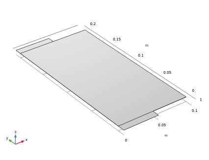
On the object fin, select Domain 1 only.
Positive Current Collector
1
In the Geometry toolbar, click  Selections and choose Explicit Selection.
2
In the Settings window for Explicit Selection, type Positive Current Collector in the Label text field.
3
On the object fin, select Domain 6 only.
Positive Electrode
1
In the Geometry toolbar, click  Selections and choose Explicit Selection.
2
In the Settings window for Explicit Selection, type Positive Electrode in the Label text field.
3
On the object fin, select Domain 5 only.
Negative Tab
1
In the Geometry toolbar, click  Selections and choose Explicit Selection.
2
In the Settings window for Explicit Selection, type Negative Tab in the Label text field.
3
On the object fin, select Domain 7 only.
Negative Current Collector
1
In the Geometry toolbar, click  Selections and choose Explicit Selection.
2
In the Settings window for Explicit Selection, type Negative Current Collector in the Label text field.
3
On the object fin, select Domain 2 only.
Negative Electrode
1
In the Geometry toolbar, click  Selections and choose Explicit Selection.
2
In the Settings window for Explicit Selection, type Negative Electrode in the Label text field.
3
On the object fin, select Domain 3 only.
Separator
1
In the Geometry toolbar, click  Selections and choose Explicit Selection.
2
In the Settings window for Explicit Selection, type Separator in the Label text field.
3
On the object fin, select Domain 4 only.
Negative Tab End
1
In the Geometry toolbar, click  Selections and choose Explicit Selection.
2
In the Settings window for Explicit Selection, type Negative Tab End in the Label text field.
3
Locate the Entities to Select section. From the Geometric entity level list, choose Boundary.
4
Click the  Paste Selection button for Entities to select.
5
In the Paste Selection dialog, type 29 in the Selection text field.
6
Positive Tab End
1
In the Geometry toolbar, click  Selections and choose Explicit Selection.
2
In the Settings window for Explicit Selection, type Positive Tab End in the Label text field.
3
Locate the Entities to Select section. From the Geometric entity level list, choose Boundary.
4
Click the  Paste Selection button for Entities to select.
5
In the Paste Selection dialog, type 2 in the Selection text field.
6
Negative Current Collector and Tab
1
In the Geometry toolbar, click  Selections and choose Union Selection.
2
In the Settings window for Union Selection, type Negative Current Collector and Tab in the Label text field.
3
Locate the Input Entities section. Click  Add.
4
In the Add dialog, in the Selections to add list, choose Negative Tab and Negative Current Collector.
5
Positive Current Collector and Tab
1
In the Geometry toolbar, click  Selections and choose Union Selection.
2
In the Settings window for Union Selection, type Positive Current Collector and Tab in the Label text field.
3
Locate the Input Entities section. Click  Add.
4
In the Add dialog, in the Selections to add list, choose Positive Tab and Positive Current Collector.
5
Metal Foil Domains
1
In the Geometry toolbar, click  Selections and choose Union Selection.
2
In the Settings window for Union Selection, type Metal Foil Domains in the Label text field.
3
Locate the Input Entities section. Click  Add.
4
In the Add dialog, in the Selections to add list, choose Negative Current Collector and Tab and Positive Current Collector and Tab.
5