COMSOL 6.4 - Discharge and Self-Discharge of a Lead

Discharge and Self-Discharge of a Lead–Acid Battery

Lead–acid batteries are widely used as starter batteries for traction applications, such as for cars and trucks. The reason for this wide usage of lead–acid batteries is their low cost in combination with their performance robustness for a broad range of operating conditions. However, one drawback of this battery type is that the inherent thermodynamics of the battery chemistry causes the battery to self-discharge over time.

This example simulates a lead–acid battery at high (1200 A) and low (3 A) discharge rates, and the long-term self-discharge behavior with no applied external current (0 A).

Figure 1: Modeled geometry. The model is in 1D in the x direction.

Model Definition

Figure 1 shows the 1D model geometry. There are four domains: the positive porous electrode, the reservoir, the separator, and the negative porous electrode.

The model uses the Lead–Acid Battery interface for solving for the following unknown variables:

•

— the electronic potential

•

— the ionic potential

•

ε — the porosity (electrolyte volume fraction) of the porous electrodes

•

cl — the electrolyte concentration

Electrochemical reactions

The main electrode reaction in the positive (PbO2) electrode during discharge is

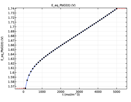
with an equilibrium potential that depends on the electrolyte concentration as shown in Figure 2.

Figure 2: Equilibrium potential of the PbO2 reaction as a function of electrolyte concentration in the positive electrode.

The combination of an aqueous solution and a high potential results in oxygen gas evolution at the positive electrode according to:

The main discharge reaction for the negative (Pb) electrode is:

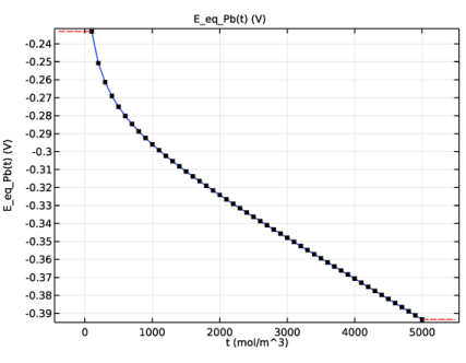
with an equilibrium potential that depends on the electrolyte concentration as shown in Figure 3.

Figure 3: Equilibrium potential of the Pb reaction as a function of electrolyte concentration in the negative electrode.

This dependence of the equilibrium potential on the electrolyte concentration, for both discharge reactions, is present in the Materials Library for the Battery Design Module.

The low operating potential of the negative electrode results in hydrogen evolution according to:

For the gas evolution reaction, Butler–Volmer type kinetic expressions are used. For the main discharge reactions the default discharge reactions of the Lead–Acid Battery interface are used.

Electrolyte transport Parameters

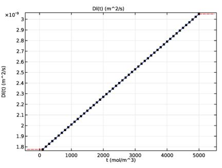
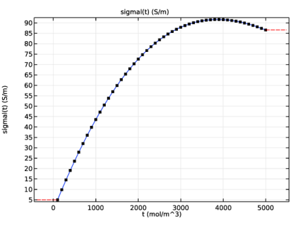
The electrolyte diffusion coefficient and the electrolyte conductivity vary with the concentration according to Figure 4 and Figure 5, respectively. This data is also present in the Materials Library for the Battery Design Module.

Figure 4: Electrolyte diffusion coefficient as a function of electrolyte concentration.

Figure 5: Electrolyte conductivity as a function of electrolyte concentration.

Boundary and initial conditions

The outer boundary of the negative electrode is grounded and a discharge current is applied to the positive end terminal.

Three different discharge currents are simulated in three separate studies. The first study performs a C/20-discharge — a constant current in order to obtain a full discharge in 20 hours, followed by a one-hour relaxation period at zero external load. The second study simulates a high load 20C-discharge during 1 minute. In the third study the external load is set to zero and the simulation time is extended to one year to study the self-discharge behavior.

Results and Discussion

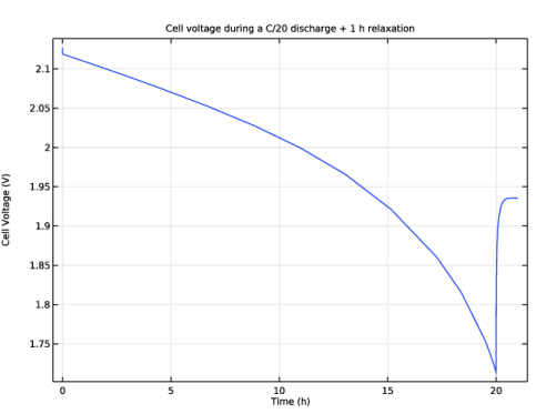
Figure 6 shows the polarization plot of the cell. At the shut-off of the current the cell voltage first rises swiftly due to the sudden absence of activation and resistive losses, but after this the potential continues to rise slightly during a relaxation period.

Figure 6: Cell voltage versus time for a C/20 discharge + 1-hour resting period.

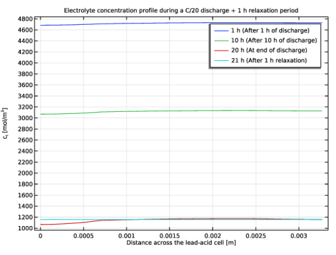
Figure 7 depicts the reason for the slow rise in potential during the resting period. When the current is cut off at 20 h there is an electrolyte concentration gradient in the cell, but as electrolyte diffuses into the electrodes during the resting period the cell potential rises slightly.

Figure 7: Electrolyte concentration profile at certain times during the C/20 discharge + 1-hour relaxation simulation.

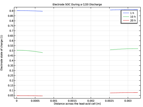
Figure 8 shows the state-of-charge variation in the electrodes during the C/20 simulation. At this relatively low discharge current the electrodes are discharged quite uniformly.

Figure 8: State-of-charge in the electrodes at 1, 10, and 20 h during the C/20 simulation.

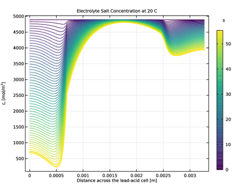
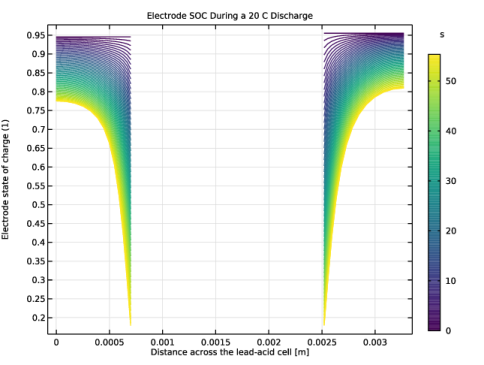
When performing the 20C simulation the concentration (Figure 9) and state-of-charge gradients (Figure 10) are much higher. These very high currents causes the battery voltage to drop significantly already after one minute due to electrolyte depletion in the positive electrode (even though two-thirds of the active electrode material is left in the electrodes).

Figure 9: Electrolyte concentration profile (one profile curve per second) during a 20C discharge until cell voltage falls below 1.5 V.

Figure 10: State-of-charge decrease during the 20C discharge simulation.

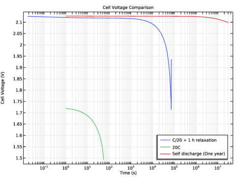
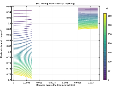
Figure 11 compares the discharge curves of the three simulations on a log t scale. The 20C cell voltage is much lower than the C/20 curve due to higher internal resistive and activation losses. The self-discharge curve indicates a moderate cell voltage drop after a year. Figure 12 shows that the state-of-charge of the positive electrode has decreased by over 25% during the same period.