|
|
|
|
•
|
|
•
|
|
•
|


|
1
|
|
2
|
|
3
|
Click Add.
|
|
4
|
Click
|
|
5
|
|
6
|
Click
|
|
1
|
|
2
|
|
3
|
Click
|
|
4
|
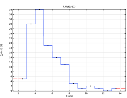
Browse to the model’s Application Libraries folder and double-click the file particle_size_distribution_parameters.txt.
|
|
1
|
|
2
|
In the Settings window for Interpolation, type Interpolation - Particle Radius Histogram in the Label text field.
|
|
3
|
|
4
|
Click
|
|
5
|
Browse to the model’s Application Libraries folder and double-click the file particle_size_distribution_histogram.txt.
|
|
6
|
Locate the Interpolation and Extrapolation section. From the Interpolation list, choose Nearest neighbor.
|
|
7
|
|
8
|
In the Argument table, enter the following settings:
|
|
9
|
|
10
|
|
11
|
|
12
|
|
13
|
Click OK.
|
|
1
|
|
2
|
In the Settings window for State Variables, type State Variables - Particle Measures From Histogram in the Label text field.
|
|
3
|
Locate the State Components section. In the table, enter the following settings:
|
|
4
|
|
1
|
|
2
|
|
3
|
|
4
|
|
5
|
|
1
|
|
2
|
|
3
|
Click
|
|
4
|
Browse to the model’s Application Libraries folder and double-click the file particle_size_distribution_variables.txt.
|
|
1
|
|
2
|
|
3
|
|
5
|
|
6
|
|
1
|
|
2
|
Go to the Add Material window.
|
|
3
|
|
4
|
Right-click and choose Add to Component 1 (comp1).
|
|
5
|
In the tree, select Battery > Electrodes > NMC 111, LiNi0.33Mn0.33Co0.33O2 (Positive, Li-ion Battery).
|
|
6
|
Right-click and choose Add to Component 1 (comp1).
|
|
7
|
|
8
|
Right-click and choose Add to Component 1 (comp1).
|
|
9
|
|
1
|
|
2
|
|
1
|
In the Model Builder window, click NMC 111, LiNi0.33Mn0.33Co0.33O2 (Positive, Li-ion Battery) (mat2).
|
|
1
|
|
1
|
In the Model Builder window, under Component 1 (comp1) > Lithium-Ion Battery (liion) click Separator 1.
|
|
2
|
|
3
|
|
1
|
|
2
|
In the Settings window for Electrode Surface, type Electrode Surface - Lithium Metal in the Label text field.
|
|
1
|
|
2
|
In the Settings window for Porous Electrode, type Porous Electrode - No Particle Size Distribution in the Label text field.
|
|
4
|
Locate the Electrolyte Properties section. From the Electrolyte material list, choose LiPF6 in 3:7 EC:EMC (Liquid, Li-ion Battery) (mat3).
|
|
5
|
|
6
|
|
7
|
|
1
|
|
2
|
|
3
|
|
4
|
|
1
|
|
2
|
|
3
|
|
4
|
Locate the Active Specific Surface Area section. From the Active specific surface area list, choose User defined. In the av text field, type Av_no_distr.
|
|
1
|
|
3
|
|
4
|
|
1
|
|
2
|
|
3
|
|
1
|
|
2
|
In the Settings window for Study, type Study 1 - No Particle Size Distribution in the Label text field.
|
|
3
|
|
1
|
In the Model Builder window, under Study 1 - No Particle Size Distribution click Step 1: Time Dependent.
|
|
2
|
|
3
|
|
4
|
|
1
|
|
2
|
|
3
|
|
5
|
Click Replace Expression in the upper-right corner of the Expression section. From the menu, choose Component 1 (comp1) > Lithium-Ion Battery > phis - Electric potential - V.
|
|
6
|
Locate the Expression section.
|
|
7
|
|
8
|
|
9
|
Click
|
|
1
|
|
2
|
|
3
|
|
5
|
Click Replace Expression in the upper-right corner of the Expression section. From the menu, choose Component 1 (comp1) > Lithium-Ion Battery > Particle intercalation > liion.cs_surface - Insertion particle concentration, surface - mol/m³.
|
|
6
|
Locate the Expression section.
|
|
7
|
|
8
|
|
9
|
|
1
|
|
2
|
|
3
|
Click Replace Expression in the upper-right corner of the Expression section. From the menu, choose Component 1 (comp1) > Lithium-Ion Battery > Particle intercalation > liion.cs_center - Insertion particle concentration, center - mol/m³.
|
|
4
|
|
1
|
|
2
|
|
3
|
|
4
|
|
5
|
|
6
|
|
7
|
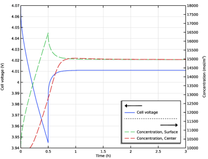
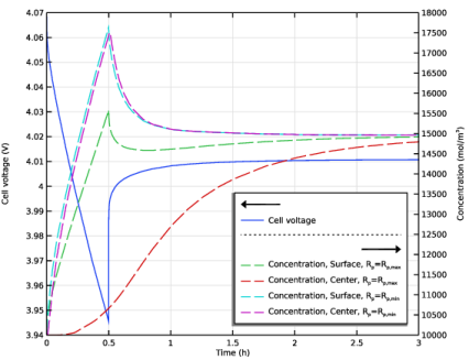
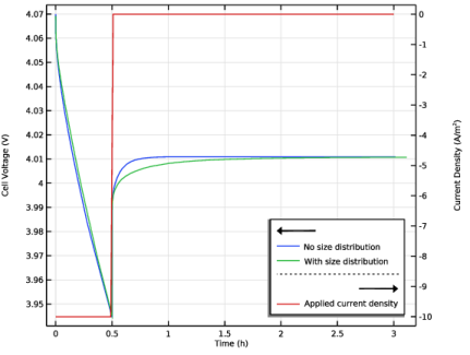
Select the Secondary y-axis label checkbox. In the associated text field, type Concentration (mol/m<sup>3</sup>).
|
|
8
|
|
9
|
|
10
|
|
11
|
|
12
|
|
13
|
|
14
|
|
15
|
|
1
|
|
2
|
|
3
|
|
1
|
|
2
|
|
3
|
|
4
|
|
6
|
|
1
|
|
2
|
Find the Spatial frame coordinates subsection. In the table, enter the following settings:
|
|
1
|
|
2
|
Click
|
|
3
|
|
4
|
|
1
|
|
3
|
|
4
|
|
1
|
|
3
|
|
4
|
|
5
|
|
6
|
|
7
|
|
1
|
In the Model Builder window, expand the Global Definitions > Extra Dimension 1 (xdim1) > Definitions node.
|
|
2
|
Right-click Global Definitions > Extra Dimension 1 (xdim1) > Definitions > Extra Dimensions and choose Integration over Extra Dimension.
|
|
3
|
In the Settings window for Integration over Extra Dimension, type Integration over Extra Dimension - xdint_surf in the Label text field.
|
|
4
|
|
5
|
|
1
|
|
2
|
In the Settings window for Integration over Extra Dimension, type Integration over Extra Dimension - xdint_surf_Rmax in the Label text field.
|
|
3
|
|
4
|
|
1
|
|
2
|
In the Settings window for Integration over Extra Dimension, type Integration over Extra Dimension - xdint_surf_Rmin in the Label text field.
|
|
3
|
|
4
|
|
1
|
|
2
|
In the Settings window for Integration over Extra Dimension, type Integration over Extra Dimension - xdint_center_Rmax in the Label text field.
|
|
3
|
|
4
|
|
1
|
|
2
|
In the Settings window for Integration over Extra Dimension, type Integration over Extra Dimension - xdint_center_Rmin in the Label text field.
|
|
3
|
|
4
|
|
1
|
In the Model Builder window, under Component 1 (comp1) right-click Definitions and choose Extra Dimensions > Attached Dimensions.
|
|
2
|
|
3
|
|
5
|
|
6
|
|
7
|
Click OK.
|
|
1
|
|
2
|
In the Settings window for Variables, type Variables - Particle Domain in Extra Dimension in the Label text field.
|
|
3
|
|
5
|
|
6
|
Locate the Variables section. In the table, enter the following settings:
|
|
1
|
|
2
|
In the Settings window for Variables, type Variables - Particle Surface in Extra Dimension in the Label text field.
|
|
3
|
|
5
|
|
6
|
|
8
|
|
9
|
Browse to the model’s Application Libraries folder and double-click the file particle_size_distribution_xdim_variables.txt.
|
|
1
|
|
2
|
In the Settings window for Variables, type Variables - Porous Electrode Domain in the Label text field.
|
|
3
|
Locate the Variables section. In the table, enter the following settings:
|
|
4
|
|
5
|
|
6
|
|
7
|
Click OK.
|
|
1
|
|
2
|
In the Settings window for Weak Contribution, type Weak Contribution - Domain Equation in Extra Dimension in the Label text field.
|
|
4
|
Locate the Domain Selection section. From the Extra dimension attachment list, choose Attached Dimensions 1.
|
|
5
|
|
6
|
Locate the Weak Contribution section. In the Weak expression text field, type xs^2*(-Rp^2*test(cs)*d(cs,TIME)-d(cs,xs)*Ds*test(d(cs,xs)[m^2])).
|
|
1
|
|
2
|
In the Settings window for Auxiliary Dependent Variable, type Auxiliary Dependent Variable - cs in the Label text field.
|
|
3
|
Locate the Domain Selection section. From the Extra dimension attachment list, choose Attached Dimensions 1.
|
|
4
|
|
5
|
|
6
|
|
1
|
|
2
|
In the Settings window for Weak Contribution, type Weak Contribution - Boundary Condition in Extra Dimension in the Label text field.
|
|
4
|
Locate the Domain Selection section. From the Extra dimension attachment list, choose Attached Dimensions 1.
|
|
5
|
|
7
|
Locate the Weak Contribution section. In the Weak expression text field, type xs^2*(-iloc/F_const)*test(cs)*Rp.
|
|
1
|
In the Model Builder window, right-click Porous Electrode - No Particle Size Distribution and choose Duplicate.
|
|
2
|
In the Settings window for Porous Electrode, type Porous Electrode - With Particle Size Distribution in the Label text field.
|
|
3
|
|
1
|
In the Model Builder window, expand the Porous Electrode - With Particle Size Distribution node, then click Porous Electrode Reaction 1.
|
|
2
|
|
3
|
|
4
|
|
1
|
|
2
|
|
3
|
|
5
|
Click Replace Expression in the upper-right corner of the Expression section. From the menu, choose Component 1 (comp1) > Lithium-Ion Battery > phis - Electric potential - V.
|
|
6
|
Locate the Expression section.
|
|
7
|
|
8
|
|
9
|
Click
|
|
1
|
|
2
|
|
3
|
|
5
|
|
6
|
Select the Description checkbox. In the associated text field, type Concentration, Surface, Largest Particles.
|
|
7
|
|
8
|
|
1
|
|
2
|
|
3
|
|
4
|
|
1
|
|
2
|
|
3
|
|
4
|
|
1
|
|
2
|
|
3
|
|
4
|
|
1
|
|
2
|
Go to the Add Study window.
|
|
3
|
|
4
|
Click the Add Study button in the window toolbar.
|
|
5
|
|
1
|
In the Model Builder window, under Study 2 - With Particle Size Distribution click Step 1: Time Dependent.
|
|
2
|
|
3
|
|
4
|
|
5
|
|
6
|
In the Probes list, choose Point Probe 1 (E_cell_no_distr), Point Probe 2 (cs_surface_no_distr), and Point Probe 3 (cs_center_no_distr).
|
|
7
|
|
8
|
Locate the Physics and Variables Selection section. Select the Modify model configuration for study step checkbox.
|
|
9
|
In the tree, select Component 1 (comp1) > Lithium-Ion Battery (liion) > Porous Electrode - No Particle Size Distribution.
|
|
10
|
Right-click and choose Disable.
|
|
11
|
|
12
|
|
13
|
Clear the Generate default plots checkbox.
|
|
14
|
|
1
|
|
2
|
|
3
|
|
4
|
|
5
|
|
6
|
|
7
|
Select the Secondary y-axis label checkbox. In the associated text field, type Concentration (mol/m<sup>3</sup>).
|
|
8
|
|
9
|
|
10
|
|
11
|
|
12
|
|
13
|
|
14
|
|
15
|
|
1
|
|
2
|
|
3
|
|
1
|
|
2
|
|
3
|
|
4
|
|
6
|
|
1
|
|
2
|
|
1
|
|
1
|
|
2
|
|
1
|
|
2
|
|
3
|
|
4
|
|
5
|
|
6
|
Locate the y-Axis Data section. In the table, enter the following settings:
|
|
1
|
|
2
|
|
3
|
|
4
|
|
5
|
|
6
|
|
7
|
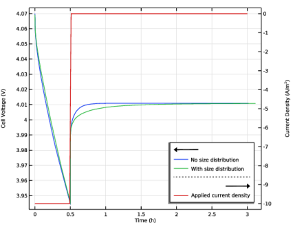
Select the Secondary y-axis label checkbox. In the associated text field, type Current Density (A/m<sup>2</sup>).
|
|
8
|
|
9
|
|
1
|
In the Model Builder window, under Results > Datasets right-click Study 2 - With Particle Size Distribution/Solution 2 (sol2) and choose Duplicate.
|
|
2
|
In the Settings window for Solution, type Study 2 - With Particle Size Distribution/Solution - xdim in the Label text field.
|
|
3
|
|
1
|
|
2
|
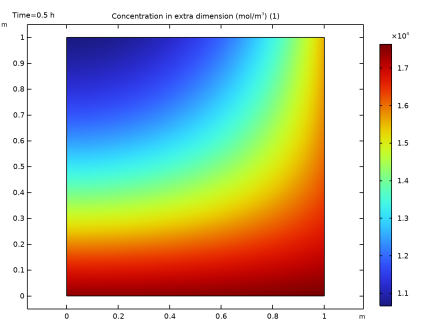
In the Settings window for 2D Plot Group, type Concentration Distribution in Particles Adjacent to Separator in the Label text field.
|
|
3
|
|
1
|
|
2
|
|
3
|
|
4
|
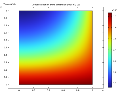
Select the Description checkbox. In the associated text field, type Concentration in extra dimension (mol/m<sup>3</sup>).
|
|
5
|
|
1
|
In the Model Builder window, right-click Concentration Distribution in Particles Adjacent to Separator and choose Duplicate.
|
|
2
|
In the Settings window for 2D Plot Group, type Concentration Distribution in Particles Adjacent to Current Collector in the Label text field.
|
|
1
|
In the Model Builder window, expand the Concentration Distribution in Particles Adjacent to Current Collector node, then click Surface 1.
|
|
2
|
|
3
|
|
4
|
|
1
|
In the Model Builder window, under Study 1 - No Particle Size Distribution click Step 1: Time Dependent.
|
|
2
|
|
3
|
|
4
|
In the Probes list, choose Point Probe 4 (E_cell_distr), Point Probe 5 (cs_surface_Rmax), Point Probe 6 (cs_center_Rmax), Point Probe 7 (cs_surface_Rmin), and Point Probe 8 (cs_center_Rmin).
|
|
5
|
|
6
|
Locate the Physics and Variables Selection section. Select the Modify model configuration for study step checkbox.
|
|
7
|
In the tree, select Component 1 (comp1) > Lithium-Ion Battery (liion) > Weak Contribution - Domain Equation in Extra Dimension.
|
|
8
|
Right-click and choose Disable.
|
|
9
|
In the tree, select Component 1 (comp1) > Lithium-Ion Battery (liion) > Weak Contribution - Boundary Condition in Extra Dimension.
|
|
10
|
Right-click and choose Disable.
|
|
11
|
In the tree, select Component 1 (comp1) > Lithium-Ion Battery (liion) > Porous Electrode - With Particle Size Distribution.
|
|
12
|
Right-click and choose Disable.
|