|
|
•
|
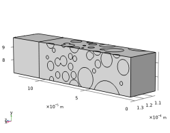
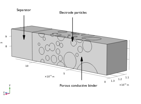
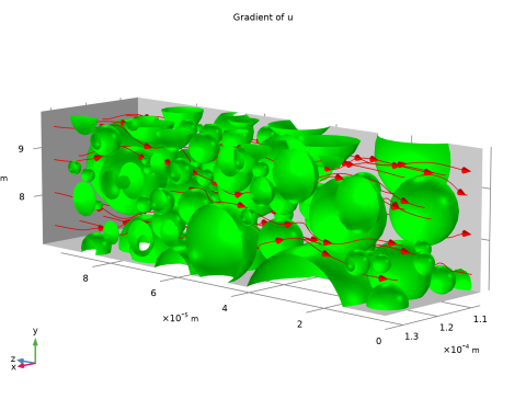
The Porous Electrode node is used to define the homogenized mixture of electrode particles, binder, and electrolyte material of the electrode, considering the volume fractions of the electrode and electrolyte phases in the 3D geometry and the effective flux parameter feff.
|
|
•
|
A Porous Electrode Reaction child node to the Porous Electrode defines the equilibrium potential, and the electrode kinetics using a specific surface area parameter based on the 3D geometry.
|
|
•
|
The diffusion of solid lithium is solved for using an extra dimension defined by the Particle Intercalation child node to the Porous Electrode, using an average particle radius that was calculated by the model method when creating the 3D geometry. (In the Heterogeneous NMC Electrode tutorial a separate Transport of Diluted Species interface was used to model the intercalated lithium diffusion.)
|
|
1
|
|
2
|
In the Application Libraries window, select Battery Design Module > Heterogeneous Models > nmc_electrode_geometry in the tree.
|
|
3
|
Click
|
|
1
|
|
2
|
|
3
|
|
1
|
|
2
|
Go to the Add Physics window.
|
|
3
|
|
4
|
Click the Add to Component 1 button in the window toolbar.
|
|
5
|
|
1
|
|
2
|
|
1
|
|
1
|
|
3
|
In the Settings window for Dirichlet Boundary Condition, locate the Dirichlet Boundary Condition section.
|
|
4
|
|
1
|
|
2
|
|
3
|
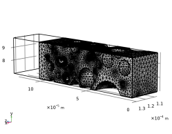
From the list, choose User-controlled mesh.
|
|
1
|
|
2
|
|
3
|
|
4
|
|
5
|
|
1
|
|
2
|
Go to the Add Study window.
|
|
3
|
|
4
|
Click the Add Study button in the window toolbar.
|
|
5
|
|
1
|
|
2
|
|
1
|
|
2
|
|
1
|
|
3
|
|
4
|
|
5
|
|
1
|
|
2
|
|
3
|
|
4
|
|
5
|
|
6
|
|
1
|
|
2
|
|
3
|
|
4
|
|
1
|
|
2
|
|
3
|
|
4
|
|
5
|
|
6
|
|
1
|
|
3
|
|
1
|
|
2
|
|
3
|
Clear the Plot dataset edges checkbox.
|
|
4
|
|
1
|
|
2
|
In the Settings window for Surface Average, type Surface Average - Effective Flux Factor in the Label text field.
|
|
4
|
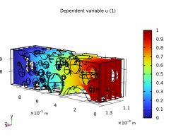
Click Replace Expression in the upper-right corner of the Expressions section. From the menu, choose Component 1 (comp1) > Laplace’s Equation > dflux.u - Boundary flux down direction - 1/m.
|
|
5
|
Locate the Expressions section. In the table, enter the following settings:
|
|
6
|
Click
|
|
1
|
|
2
|
|
1
|
|
2
|
|
3
|
|
4
|
Browse to the model’s Application Libraries folder and double-click the file nmc_electrode_parameters.txt.
|
|
1
|
|
2
|
|
3
|
|
5
|
|
1
|
|
2
|
Go to the Add Physics window.
|
|
3
|
|
4
|
Click the Add to Component 2 button in the window toolbar.
|
|
5
|
|
1
|
|
2
|
Go to the Add Material window.
|
|
3
|
In the tree, select Battery > Electrodes > NMC 111, LiNi0.33Mn0.33Co0.33O2 (Positive, Li-ion Battery).
|
|
4
|
Right-click and choose Add to Component 2 (comp2).
|
|
5
|
|
6
|
Right-click and choose Add to Component 2 (comp2).
|
|
7
|
|
8
|
Right-click and choose Add to Component 2 (comp2).
|
|
9
|
|
1
|
|
2
|
|
1
|
|
2
|
|
3
|
|
1
|
|
2
|
|
3
|
|
1
|
In the Model Builder window, under Component 2 (comp2) > Lithium-Ion Battery (liion) click Separator 1.
|
|
2
|
|
3
|
|
1
|
|
3
|
|
4
|
|
5
|
|
6
|
|
7
|
Locate the Effective Transport Parameter Correction section. From the Electrolyte conductivity list, choose User defined. In the fl text field, type f_eff*(eps_l_b^1.5).
|
|
8
|
|
9
|
|
1
|
|
2
|
|
3
|
From the Particle material list, choose NMC 111, LiNi0.33Mn0.33Co0.33O2 (Positive, Li-ion Battery) (mat1).
|
|
4
|
|
5
|
|
1
|
|
2
|
|
3
|
|
4
|
|
5
|
Locate the Active Specific Surface Area section. From the Active specific surface area list, choose User defined. In the av text field, type Av_particles.
|
|
1
|
|
1
|
|
2
|
|
3
|
|
1
|
|
3
|
|
4
|
|
1
|
|
2
|
|
3
|
|
5
|
|
1
|
|
2
|
Go to the Add Study window.
|
|
3
|
Find the Studies subsection. In the Select Study tree, select Preset Studies for Some Physics Interfaces > Time Dependent with Initialization.
|
|
4
|
Right-click and choose Add Study.
|
|
5
|
|
1
|
In the Settings window for Current Distribution Initialization, locate the Physics and Variables Selection section.
|
|
2
|
In the Solve for column of the table, under Component 1 (comp1), clear the checkbox for Laplace’s Equation (lpeq).
|
|
3
|
Click to expand the Mesh Selection section. Disabling the mesh in Geometry 1, which is not used by the homogenized model, memory can be saved.
|
|
1
|
|
2
|
|
3
|
|
4
|
|
5
|
Locate the Physics and Variables Selection section. In the Solve for column of the table, under Component 1 (comp1), clear the checkbox for Laplace’s Equation (lpeq).
|
|
6
|
Click to expand the Mesh Selection section. In the table, enter the following settings:
|
|
1
|
|
2
|
|
3
|
|
4
|
|
5
|
Right-click Study 2 > Solver Configurations > Solution 2 (sol2) > Time-Dependent Solver 1 and choose Stop Condition.
|
|
6
|
|
7
|
Click
|
|
9
|
|
10
|
|
1
|
|
1
|
|
2
|
In the Settings window for Porous Matrix Double Layer Capacitance, locate the Porous Matrix Double Layer Capacitance section.
|
|
3
|
|
4
|
|
1
|
In the Model Builder window, under Component 2 (comp2) > Lithium-Ion Battery (liion) right-click Electrode Current 1 and choose Duplicate.
|
|
2
|
In the Settings window for Electrode Current, type Electrode Current - Harmonic Perturbation in the Label text field.
|
|
3
|
|
1
|
|
2
|
|
3
|
|
1
|
|
2
|
|
1
|
|
2
|
Go to the Add Study window.
|
|
3
|
Find the Studies subsection. In the Select Study tree, select Preset Studies for Some Physics Interfaces > AC Impedance, Initial Values.
|
|
4
|
Right-click and choose Add Study.
|
|
5
|
|
1
|
|
2
|
|
3
|
Locate the Physics and Variables Selection section. In the Solve for column of the table, under Component 1 (comp1), clear the checkbox for Laplace’s Equation (lpeq).
|
|
4
|
Click to expand the Mesh Selection section. In the table, enter the following settings:
|
|
1
|
In the Study toolbar, click
|
|
2
|
|
3
|
In the Settings window for Current Distribution Initialization, locate the Physics and Variables Selection section.
|
|
4
|
In the Solve for column of the table, under Component 1 (comp1), clear the checkbox for Laplace’s Equation (lpeq).
|
|
5
|
Locate the Mesh Selection section. In the table, enter the following settings:
|
|
6
|
|
1
|
|
2
|
In the Settings window for Table, type Heterogeneous Discharge Data (Imported) in the Label text field.
|
|
3
|
|
4
|
Browse to the model’s Application Libraries folder and double-click the file nmc_electrode_heterogeneous_discharge_data.txt.
|
|
1
|
|
2
|
|
3
|
|
4
|
Browse to the model’s Application Libraries folder and double-click the file nmc_electrode_heterogeneous_eis_data.txt.
|
|
1
|
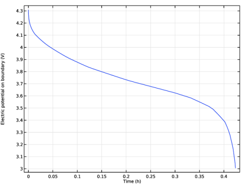
In the Model Builder window, under Results click Boundary Electrode Potential with Respect to Ground (liion).
|
|
2
|
|
3
|
Locate the Plot Settings section.
|
|
4
|
|
5
|
|
1
|
|
2
|
|
3
|
|
4
|
|
5
|
|
1
|
|
2
|
|
3
|
|
5
|
|
1
|
In the Model Builder window, expand the Results > Impedance with Respect to Ground, Nyquist (liion) node, then click Impedance with Respect to Ground, Nyquist (liion).
|
|
2
|
|
3
|
|
4
|
|
5
|
|
1
|
|
2
|
|
3
|
|
4
|
|
5
|
|
6
|
|
7
|
|
8
|
|
10
|
|
1
|
|
2
|
|
3
|
|
5
|