
|
|
|
|
•
|
|
•
|
|
•
|
|
•
|
|
•
|
Electrolyte: 1.0 M NaPF6 dissolved in EC:PC (0.5:0.5 w/w)
|

|
1
|
|
2
|
|
3
|
Click Add.
|
|
4
|
Click
|
|
5
|
In the Select Study tree, select Preset Studies for Selected Physics Interfaces > Time Dependent with Initialization.
|
|
6
|
Click
|
|
1
|
|
2
|
|
3
|
Click
|
|
4
|
Browse to the model’s Application Libraries folder and double-click the file na_ion_battery_1d_parameters.txt.
|
|
1
|
|
2
|
|
3
|
|
5
|
Click
|
|
1
|
|
2
|
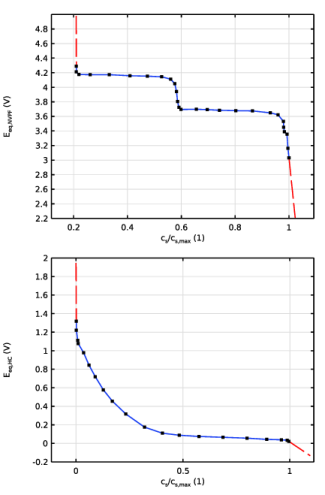
In the Settings window for Interpolation, type Interpolation - Eeq_NVPF (Positive Electrode) in the Label text field.
|
|
3
|
|
4
|
Click
|
|
5
|
Browse to the model’s Application Libraries folder and double-click the file na_ion_battery_1d_Eeq_NVPF.txt.
|
|
6
|
|
7
|
|
8
|
In the Argument table, enter the following settings:
|
|
1
|
|
2
|
In the Settings window for Interpolation, type Interpolation - Eeq_HC (Negative Electrode) in the Label text field.
|
|
3
|
|
4
|
Click
|
|
5
|
Browse to the model’s Application Libraries folder and double-click the file na_ion_battery_1d_Eeq_HC.txt.
|
|
6
|
|
7
|
|
8
|
In the Argument table, enter the following settings:
|
|
1
|
|
2
|
|
3
|
|
4
|
Click
|
|
5
|
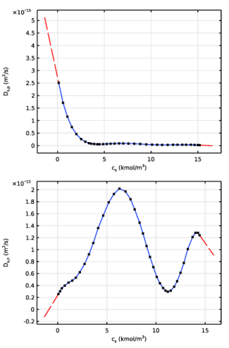
Browse to the model’s Application Libraries folder and double-click the file na_ion_battery_1d_Ds_p.txt.
|
|
6
|
|
7
|
|
8
|
In the Argument table, enter the following settings:
|
|
1
|
|
2
|
|
3
|
|
4
|
Click
|
|
5
|
Browse to the model’s Application Libraries folder and double-click the file na_ion_battery_1d_Ds_n.txt.
|
|
6
|
|
7
|
|
8
|
In the Argument table, enter the following settings:
|
|
1
|
|
2
|
|
3
|
|
4
|
Click
|
|
5
|
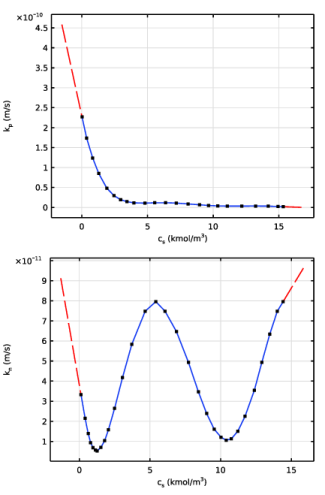
Browse to the model’s Application Libraries folder and double-click the file na_ion_battery_1d_k_p.txt.
|
|
6
|
|
7
|
|
8
|
In the Argument table, enter the following settings:
|
|
1
|
|
2
|
|
3
|
|
4
|
Click
|
|
5
|
Browse to the model’s Application Libraries folder and double-click the file na_ion_battery_1d_k_n.txt.
|
|
6
|
|
7
|
|
8
|
In the Argument table, enter the following settings:
|
|
1
|
|
2
|
|
3
|
|
4
|
Click
|
|
5
|
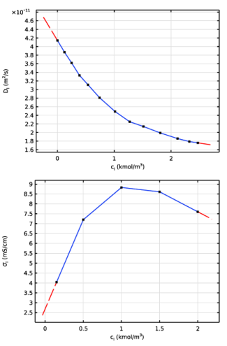
Browse to the model’s Application Libraries folder and double-click the file na_ion_battery_1d_Dl.txt.
|
|
6
|
|
7
|
|
8
|
In the Argument table, enter the following settings:
|
|
1
|
|
2
|
|
3
|
|
4
|
Click
|
|
5
|
Browse to the model’s Application Libraries folder and double-click the file na_ion_battery_1d_sigmal.txt.
|
|
6
|
|
7
|
|
8
|
In the Argument table, enter the following settings:
|
|
1
|
|
2
|
|
3
|
|
1
|
|
2
|
|
3
|
|
1
|
|
2
|
|
3
|
Click
|
|
4
|
Browse to the model’s Application Libraries folder and double-click the file na_ion_battery_1d_variables.txt.
|
|
1
|
|
2
|
|
3
|
|
1
|
In the Model Builder window, under Component 1 (comp1) > Sodium-Ion Battery (liion) click Separator 1.
|
|
2
|
|
3
|
|
4
|
|
5
|
|
6
|
|
7
|
|
1
|
|
3
|
|
4
|
|
5
|
|
6
|
|
7
|
|
8
|
|
9
|
|
10
|
|
11
|
Locate the Effective Transport Parameter Correction section. From the Electric conductivity list, choose No correction.
|
|
1
|
|
2
|
|
3
|
|
4
|
|
5
|
Locate the Particle Transport Properties section. From the Ds list, choose User defined. In the associated text field, type Ds_n(liion.cs_pce1).
|
|
6
|
|
7
|
Click to expand the Operational SOCs for Initial Cell Charge Distribution section. From the socmin list, choose User defined. From the socmax list, choose User defined.
|
|
1
|
|
2
|
|
3
|
From the Eeq list, choose User defined. In the associated text field, type Eeq_HC(liion.cs_surface/csmax_n).
|
|
4
|
Locate the Electrode Kinetics section. From the Exchange current density type list, choose Rate constant.
|
|
5
|
|
6
|
|
7
|
|
8
|
|
9
|
|
1
|
|
3
|
|
4
|
|
5
|
|
6
|
|
7
|
|
8
|
|
9
|
|
10
|
|
11
|
Locate the Effective Transport Parameter Correction section. From the Electric conductivity list, choose No correction.
|
|
1
|
|
2
|
|
3
|
|
4
|
|
5
|
Locate the Particle Transport Properties section. From the Ds list, choose User defined. In the associated text field, type Ds_p(liion.cs_pce2).
|
|
6
|
|
7
|
Locate the Operational SOCs for Initial Cell Charge Distribution section. From the socmin list, choose User defined. From the socmax list, choose User defined.
|
|
1
|
|
2
|
|
3
|
From the Eeq list, choose User defined. In the associated text field, type Eeq_NVPF(liion.cs_surface/csmax_p).
|
|
4
|
Locate the Electrode Kinetics section. From the Exchange current density type list, choose Rate constant.
|
|
5
|
|
6
|
|
7
|
|
8
|
|
9
|
|
1
|
|
3
|
|
4
|
Select the Include contact resistance checkbox.
|
|
5
|
|
1
|
|
3
|
|
4
|
From the list, choose Average current density.
|
|
5
|
|
6
|
|
7
|
|
8
|
|
1
|
|
2
|
|
3
|
|
1
|
|
2
|
|
3
|
|
4
|
|
1
|
|
2
|
|
3
|
Click
|
|
1
|
|
2
|
|
3
|
|
4
|
|
5
|
|
1
|
|
2
|
|
3
|
|
4
|
|
5
|
|
6
|
Right-click Study 1 > Solver Configurations > Solution 1 (sol1) > Time-Dependent Solver 1 and choose Stop Condition.
|
|
7
|
|
8
|
Click
|
|
10
|
|
11
|
Clear the Add information checkbox.
|
|
12
|
|
1
|
|
2
|
|
3
|
|
1
|
|
2
|
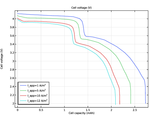
In the Settings window for 1D Plot Group, type Cell Voltage vs. Cell Capacity in the Label text field.
|
|
3
|
|
1
|
|
2
|
|
4
|
Click Replace Expression in the upper-right corner of the y-Axis Data section. From the menu, choose Component 1 (comp1) > Definitions > Variables > E_cell - Cell voltage - V.
|
|
5
|
|
6
|
|
7
|
|
8
|
|
9
|
|
1
|
|
2
|
|
3
|
|
4
|
|
1
|
|
2
|
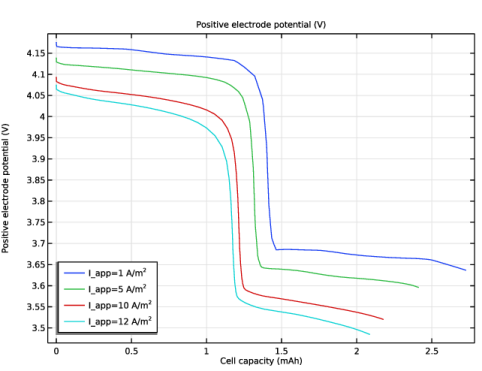
In the Settings window for 1D Plot Group, type Positive Electrode Potential vs. Cell Capacity in the Label text field.
|
|
1
|
In the Model Builder window, expand the Positive Electrode Potential vs. Cell Capacity node, then click Global 1.
|
|
2
|
In the Settings window for Global, click Replace Expression in the upper-right corner of the y-Axis Data section. From the menu, choose Component 1 (comp1) > Definitions > Variables > E_pos - Positive electrode potential - V.
|
|
1
|
|
2
|
|
1
|
|
2
|
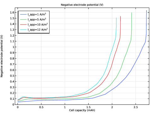
In the Settings window for 1D Plot Group, type Negative Electrode Potential vs. Cell Capacity in the Label text field.
|
|
1
|
In the Model Builder window, expand the Negative Electrode Potential vs. Cell Capacity node, then click Global 1.
|
|
2
|
In the Settings window for Global, click Replace Expression in the upper-right corner of the y-Axis Data section. From the menu, choose Component 1 (comp1) > Definitions > Variables > E_neg - Negative electrode potential - V.
|
|
1
|
|
2
|
|
3
|
|
4
|