
|
|
|
|
•
|
|
•
|
|
•
|
The electrochemical reactions are dependent on the solid phase potential, ϕs, and the pseudo-potentiostatic electrolyte potential, ϕl,ps. The latter is used instead of the electrolyte phase potential variable, ϕl, and includes an ideal electrolyte concentration dependence for single charged ions (that is, the dominating charge of ions in this example). For more information, see the Copper Current-Collector Dissolution example.
|
|
1
|
|
2
|
|
3
|
Click Add.
|
|
4
|
|
5
|
Click Add.
|
|
6
|
Click
|
|
7
|
In the Select Study tree, select Preset Studies for Selected Physics Interfaces > Lithium-Ion Battery > Time Dependent with Initialization.
|
|
8
|
Click
|
|
1
|
|
2
|
|
3
|
Click
|
|
4
|
Browse to the model’s Application Libraries folder and double-click the file lmo_decomposition_parameters.txt.
|
|
1
|
|
2
|
|
4
|
Click
|
|
5
|
|
1
|
|
2
|
|
1
|
|
2
|
|
1
|
|
2
|
|
3
|
|
1
|
|
2
|
Go to the Add Material window.
|
|
3
|
|
4
|
Click the Add to Component button in the window toolbar.
|
|
5
|
|
6
|
Click the Add to Component button in the window toolbar.
|
|
7
|
|
8
|
Click the Add to Component button in the window toolbar.
|
|
9
|
|
1
|
|
2
|
|
1
|
|
2
|
|
3
|
|
1
|
|
2
|
|
3
|
|
4
|
|
1
|
|
2
|
|
3
|
|
4
|
Browse to the model’s Application Libraries folder and double-click the file lmo_decomposition_variables.txt.
|
|
1
|
|
2
|
|
3
|
|
4
|
|
5
|
|
6
|
Browse to the model’s Application Libraries folder and double-click the file lmo_decomposition_variables_lmo.txt.
|
|
1
|
|
2
|
|
3
|
|
4
|
|
1
|
|
2
|
|
3
|
|
4
|
|
1
|
|
2
|
|
3
|
Select the Define cell state of charge (SOC) and initial charge inventory checkbox.
|
|
1
|
In the Model Builder window, under Component 1 (comp1) > Lithium-Ion Battery (liion) click SOC and Initial Charge Distribution 1.
|
|
2
|
|
3
|
From the list, choose Half cell.
|
|
4
|
Locate the State-of-Charge Definition section. From the list, choose User defined. In the Ecell0%SOC text field, type Vlow.
|
|
5
|
|
6
|
|
1
|
|
2
|
In the Settings window for Positive Electrode Domain Selection, locate the Domain Selection section.
|
|
3
|
|
1
|
In the Model Builder window, under Component 1 (comp1) > Lithium-Ion Battery (liion) click Separator 1.
|
|
2
|
|
3
|
|
1
|
|
2
|
|
4
|
Locate the Electrolyte Properties section. From the Electrolyte material list, choose LiPF6 in 1:1 EC:DMC (Liquid, Li-ion Battery) (mat1).
|
|
5
|
|
6
|
|
7
|
|
8
|
|
10
|
Clear the Subtract volume change from electrolyte volume fraction checkbox.
|
|
1
|
|
2
|
In the Settings window for Particle Intercalation, locate the Particle Transport Properties section.
|
|
3
|
|
4
|
|
1
|
In the Model Builder window, under Component 1 (comp1) > Lithium-Ion Battery (liion) > Porous Electrode - LMO click Porous Electrode Reaction 1.
|
|
2
|
In the Settings window for Porous Electrode Reaction, type Porous Electrode Reaction - Intercalation in the Label text field.
|
|
3
|
|
1
|
|
2
|
In the Settings window for Porous Electrode Reaction, type Porous Electrode Reaction - Solvent Oxidation in the Label text field.
|
|
3
|
Locate the Equilibrium Potential section. From the Eeq list, choose User defined. In the associated text field, type Eeq_oxid+delta_phil.
|
|
4
|
Locate the Electrode Kinetics section. From the Kinetics expression type list, choose Anodic Tafel equation.
|
|
5
|
|
6
|
|
7
|
Locate the Active Specific Surface Area section. From the Active specific surface area list, choose User defined. In the av text field, type av_oxid.
|
|
8
|
|
1
|
|
2
|
In the Settings window for Nonfaradaic Reactions, type Nonfaradaic Reactions - LMO Decomposition in the Label text field.
|
|
3
|
Locate the Reaction Rate section. In the Reaction rate for dissolving–depositing species table, enter the following settings:
|
|
1
|
|
3
|
In the Settings window for Electrode Surface, type Electrode Surface - Lithium Metal in the Label text field.
|
|
1
|
In the Model Builder window, under Component 1 (comp1) > Lithium-Ion Battery (liion) > Electrode Surface - Lithium Metal click Electrode Reaction 1.
|
|
2
|
In the Settings window for Electrode Reaction, type Electrode Reaction - Lithium in the Label text field.
|
|
1
|
|
2
|
In the Settings window for Electrode Reaction, type Electrode Reaction - Manganese Deposition in the Label text field.
|
|
3
|
Locate the Equilibrium Potential section. From the Eeq list, choose User defined. In the associated text field, type Eeq_Mn+delta_phil.
|
|
4
|
Locate the Electrode Kinetics section. From the Kinetics expression type list, choose Cathodic Tafel equation.
|
|
5
|
|
6
|
|
7
|
|
8
|
|
1
|
|
2
|
In the Settings window for Electrode Reaction, type Electrode Reaction - Proton Reduction in the Label text field.
|
|
3
|
Locate the Equilibrium Potential section. From the Eeq list, choose User defined. In the associated text field, type Eeq_H+delta_phil.
|
|
4
|
Locate the Electrode Kinetics section. From the Kinetics expression type list, choose Cathodic Tafel equation.
|
|
5
|
|
6
|
|
7
|
|
8
|
In the Show More Options dialog, in the tree, select the checkbox for the node Physics > Advanced Physics Options.
|
|
9
|
Click OK.
|
|
1
|
|
2
|
In the Settings window for Reaction Source, type Reaction Source - Cation Net Chemical Reactions in the Label text field.
|
|
3
|
|
4
|
|
1
|
|
2
|
In the Settings window for Charge-Discharge Cycling, type Charge-Discharge Cycling - Galvanic Cycling C/3 in the Label text field.
|
|
4
|
|
5
|
|
6
|
|
7
|
|
8
|
|
9
|
|
10
|
|
1
|
|
2
|
|
3
|
Clear the Convection checkbox.
|
|
4
|
Select the Migration in electric field checkbox.
|
|
5
|
Select the Mass transfer in porous media checkbox.
|
|
6
|
Click to expand the Dependent Variables section. In the Concentrations (mol/m³) table, enter the following settings:
|
|
7
|
Click
|
|
8
|
In the Concentrations (mol/m³) table, enter the following settings:
|
|
9
|
Click
|
|
10
|
In the Concentrations (mol/m³) table, enter the following settings:
|
|
1
|
In the Model Builder window, under Component 1 (comp1) > Transport of Diluted Species (tds) click Species Charges.
|
|
2
|
|
3
|
|
4
|
|
1
|
|
2
|
|
3
|
|
1
|
|
2
|
|
3
|
|
4
|
|
5
|
|
6
|
|
7
|
|
1
|
|
2
|
|
3
|
|
1
|
|
2
|
|
3
|
|
1
|
|
2
|
|
3
|
From the iv list, choose Local current source, Porous Electrode Reaction - Solvent Oxidation (liion/pce1/per2).
|
|
4
|
|
1
|
|
2
|
|
3
|
|
1
|
|
2
|
|
3
|
|
4
|
|
5
|
|
6
|
|
7
|
|
1
|
|
2
|
|
3
|
|
1
|
|
2
|
In the Settings window for Electrode Surface Coupling, type Electrode Surface Coupling - Lithium Metal in the Label text field.
|
|
3
|
|
1
|
In the Model Builder window, expand the Electrode Surface Coupling - Lithium Metal node, then click Reaction Coefficients 1.
|
|
2
|
In the Settings window for Reaction Coefficients, type Reaction Coefficients - Manganese deposition in the Label text field.
|
|
3
|
Locate the Reaction Current Density section. From the iloc list, choose Local current density, Electrode Reaction - Manganese Deposition (liion/es1/er2).
|
|
4
|
|
5
|
|
1
|
|
2
|
In the Settings window for Reaction Coefficients, type Reaction Coefficients - Proton Reduction in the Label text field.
|
|
3
|
Locate the Reaction Current Density section. From the iloc list, choose Local current density, Electrode Reaction - Proton Reduction (liion/es1/er3).
|
|
4
|
|
1
|
|
2
|
|
3
|
|
4
|
|
5
|
|
6
|
|
1
|
|
2
|
|
3
|
|
4
|
|
5
|
|
1
|
In the Settings window for Time Dependent, type Time Dependent - First Cycle in the Label text field.
|
|
2
|
|
3
|
|
1
|
|
2
|
|
3
|
|
4
|
|
1
|
|
2
|
In the Settings window for Time Dependent, type Time Dependent - Last Cycle in the Label text field.
|
|
3
|
|
4
|
|
1
|
|
2
|
|
3
|
|
4
|
|
5
|
Right-click Study 1 > Solver Configurations > Solution 1 (sol1) > Time-Dependent Solver 1 and choose Stop Condition.
|
|
6
|
|
7
|
Click
|
|
9
|
|
10
|
In the Model Builder window, under Study 1 > Solver Configurations > Solution 1 (sol1) right-click Time-Dependent Solver 2 and choose Stop Condition.
|
|
11
|
|
12
|
Click
|
|
14
|
|
15
|
In the Model Builder window, under Study 1 > Solver Configurations > Solution 1 (sol1) click Time-Dependent Solver 3.
|
|
16
|
|
17
|
|
18
|
Right-click Study 1 > Solver Configurations > Solution 1 (sol1) > Time-Dependent Solver 3 and choose Stop Condition.
|
|
19
|
|
20
|
Click
|
|
22
|
|
23
|
|
1
|
|
2
|
|
3
|
|
4
|
|
5
|
|
6
|
|
1
|
|
2
|
|
3
|
|
4
|
|
5
|
|
6
|
|
1
|
In the Model Builder window, under Results click Cell and Average Electrode Cell State of Charge (liion).
|
|
2
|
|
3
|
|
4
|
|
1
|
In the Model Builder window, expand the Cell and Average Electrode Cell State of Charge (liion) node, then click Global 1.
|
|
2
|
|
3
|
|
4
|
|
5
|
|
1
|
|
2
|
|
3
|
|
4
|
|
5
|
|
6
|
|
1
|
In the Model Builder window, under Results, Ctrl-click to select Electrode Potential with Respect to Adjacent Reference (liion), Electrolyte Salt Concentration (liion), Volumetric Current Density (liion), Particle Surface State of Charge (liion), Concentrations, All Species (tds), Concentration, H (tds), Concentration, Mn (tds), and Concentration, H2O (tds).
|
|
2
|
Right-click and choose Delete.
|
|
1
|
|
2
|
|
3
|
|
4
|
|
5
|
|
6
|
|
1
|
|
2
|
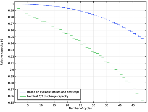
In the Settings window for Global, click Replace Expression in the upper-right corner of the y-Axis Data section. From the menu, choose Component 1 (comp1) > Lithium-Ion Battery > liion.Q_cell - Battery cell capacity - C.
|
|
3
|
Locate the y-Axis Data section. In the table, enter the following settings:
|
|
4
|
|
5
|
|
6
|
|
7
|
|
1
|
|
2
|
|
3
|
|
4
|
|
5
|
|
1
|
|
2
|
|
4
|
Click Replace Expression in the upper-right corner of the x-Axis Data section. From the menu, choose Component 1 (comp1) > Lithium-Ion Battery > Charge-Discharge Cycling - Galvanic Cycling C/3 > liion.cdc1.cycle_counter - Number of cycles.
|
|
5
|
|
1
|
|
2
|
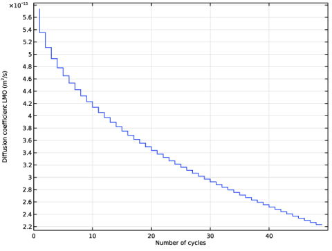
In the Settings window for 1D Plot Group, type Diffusion Coefficient in LMO Particles in the Label text field.
|
|
3
|
Locate the Plot Settings section.
|
|
4
|
Select the y-axis label checkbox. In the associated text field, type Diffusion coefficient LMO (m<sup>2</sup>/s).
|
|
1
|
In the Model Builder window, expand the Diffusion Coefficient in LMO Particles node, then click Global 1.
|
|
2
|
|
4
|
|
1
|
In the Model Builder window, right-click Diffusion Coefficient in LMO Particles and choose Duplicate.
|
|
2
|
|
3
|
|
4
|
Locate the Plot Settings section.
|
|
5
|
|
6
|
|
7
|
|
1
|
|
2
|
|
3
|
|
4
|
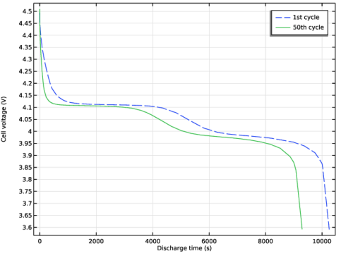
Click Replace Expression in the upper-right corner of the y-Axis Data section. From the menu, choose Component 1 (comp1) > Lithium-Ion Battery > Charge-Discharge Cycling - Galvanic Cycling C/3 > liion.cdc1.phis0 - Cell potential - V.
|
|
5
|
|
6
|
Click to expand the Coloring and Style section. Find the Line style subsection. From the Line list, choose Dashed.
|
|
7
|
|
1
|
|
2
|
|
3
|
Clear the Decreasing x checkbox.
|
|
4
|
Clear the Increasing y checkbox.
|
|
1
|
|
2
|
|
3
|
|
4
|
|
5
|
Locate the Coloring and Style section. Find the Line style subsection. From the Line list, choose Solid.
|
|
6
|
Locate the Legends section. In the table, enter the following settings:
|
|
7
|
|
1
|
In the Model Builder window, right-click Diffusion Coefficient in LMO Particles and choose Duplicate.
|
|
2
|
|
3
|
|
4
|
|
5
|
|
1
|
|
2
|
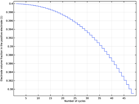
In the Settings window for Global, click Replace Expression in the upper-right corner of the y-Axis Data section. From the menu, choose Component 1 (comp1) > Lithium-Ion Battery > liion.SOH_cell - Cell state of health - 1.
|
|
3
|
|
1
|
|
2
|
|
4
|
Locate the Legends section. In the table, enter the following settings:
|
|
1
|
|
2
|
|
3
|
Clear the Decreasing x checkbox.
|
|
4
|
|
1
|
In the Model Builder window, right-click Diffusion Coefficient in LMO Particles and choose Duplicate.
|
|
2
|
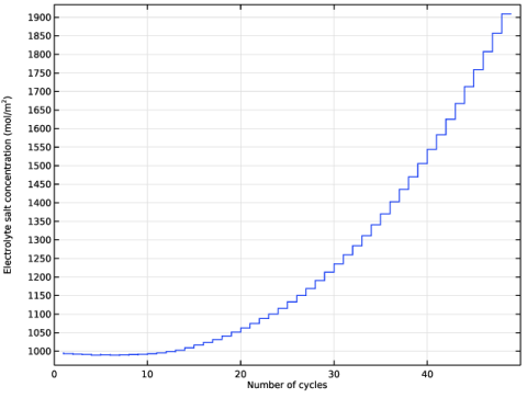
In the Settings window for 1D Plot Group, type Electrolyte Salt Concentration in Battery in the Label text field.
|
|
3
|
Locate the Plot Settings section. In the y-axis label text field, type Electrolyte salt concentration (mol/m<sup>2</sup>).
|
|
1
|
In the Model Builder window, expand the Electrolyte Salt Concentration in Battery node, then click Global 1.
|
|
2
|
|
4
|