|
|
|
|
1
|
|
2
|
In the Select Physics tree, select Electrochemistry > Tertiary Current Distribution, Nernst–Planck > Tertiary, Electroneutrality (tcd).
|
|
3
|
Click Add.
|
|
4
|
|
5
|
In the Concentrations (mol/m³) table, enter the following settings:
|
|
6
|
Click
|
|
7
|
In the Select Study tree, select Preset Studies for Selected Physics Interfaces > Time Dependent with Initialization.
|
|
8
|
Click
|
|
1
|
In the Model Builder window, under Component 1 (comp1) click Tertiary Current Distribution, Nernst–Planck (tcd).
|
|
2
|
In the Settings window for Tertiary Current Distribution, Nernst–Planck, locate the Electrolyte Charge Conservation section.
|
|
3
|
|
1
|
|
2
|
|
3
|
Click
|
|
4
|
Browse to the model’s Application Libraries folder and double-click the file lithium_sulfur_parameters.txt.
|
|
1
|
|
2
|
|
3
|
|
5
|
|
1
|
In the Model Builder window, under Component 1 (comp1) click Tertiary Current Distribution, Nernst–Planck (tcd).
|
|
2
|
In the Settings window for Tertiary Current Distribution, Nernst–Planck, locate the Cross-Sectional Area section.
|
|
3
|
|
1
|
In the Model Builder window, under Component 1 (comp1) > Tertiary Current Distribution, Nernst–Planck (tcd) click Species Charges 1.
|
|
2
|
|
3
|
|
4
|
|
5
|
|
6
|
|
7
|
|
8
|
|
9
|
|
1
|
|
3
|
|
4
|
|
5
|
|
6
|
|
7
|
|
8
|
|
9
|
|
10
|
|
11
|
|
12
|
|
1
|
|
3
|
|
4
|
|
5
|
|
6
|
|
7
|
|
8
|
|
9
|
|
10
|
|
11
|
|
12
|
Locate the Electrode Current Conduction section. From the σs list, choose User defined. In the associated text field, type sigma_s.
|
|
13
|
|
14
|
|
15
|
Locate the Effective Transport Parameter Correction section. From the Electric conductivity list, choose No correction.
|
|
1
|
|
2
|
In the Settings window for Porous Electrode Reaction, locate the Stoichiometric Coefficients section.
|
|
3
|
|
4
|
|
5
|
|
6
|
Click to expand the Reference Concentrations section. In the table, enter the following settings:
|
|
7
|
|
8
|
|
1
|
|
2
|
In the Settings window for Porous Electrode Reaction, locate the Stoichiometric Coefficients section.
|
|
3
|
|
4
|
|
5
|
|
6
|
Locate the Reference Concentrations section. In the table, enter the following settings:
|
|
7
|
|
8
|
|
1
|
|
2
|
In the Settings window for Porous Electrode Reaction, locate the Stoichiometric Coefficients section.
|
|
3
|
|
4
|
|
5
|
|
6
|
Locate the Reference Concentrations section. In the table, enter the following settings:
|
|
7
|
|
8
|
|
1
|
|
2
|
In the Settings window for Porous Electrode Reaction, locate the Stoichiometric Coefficients section.
|
|
3
|
|
4
|
|
5
|
|
6
|
Locate the Reference Concentrations section. In the table, enter the following settings:
|
|
7
|
|
8
|
|
1
|
|
2
|
In the Settings window for Porous Electrode Reaction, locate the Stoichiometric Coefficients section.
|
|
3
|
|
4
|
|
5
|
|
6
|
Locate the Reference Concentrations section. In the table, enter the following settings:
|
|
7
|
|
8
|
|
1
|
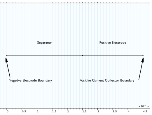
In the Model Builder window, under Component 1 (comp1) > Tertiary Current Distribution, Nernst–Planck (tcd) click Separator 1.
|
|
2
|
|
3
|
Click
|
|
5
|
Click
|
|
1
|
|
2
|
In the Settings window for Porous Electrode, click to expand the Dissolving–Depositing Species section.
|
|
3
|
Click
|
|
5
|
Click
|
|
1
|
In the Model Builder window, under Component 1 (comp1) right-click Definitions and choose Variables.
|
|
2
|
|
3
|
|
5
|
|
6
|
Browse to the model’s Application Libraries folder and double-click the file lithium_sulfur_separator_variables.txt.
|
|
1
|
|
2
|
|
3
|
|
5
|
|
6
|
Browse to the model’s Application Libraries folder and double-click the file lithium_sulfur_electrode_variables.txt.
|
|
1
|
|
2
|
|
3
|
|
4
|
Browse to the model’s Application Libraries folder and double-click the file lithium_sulfur_all_domains_variables.txt.
|
|
1
|
In the Model Builder window, under Component 1 (comp1) > Tertiary Current Distribution, Nernst–Planck (tcd) > Separator 1 click Nonfaradaic Reactions 1.
|
|
2
|
In the Settings window for Nonfaradaic Reactions, type Non-Faradaic Reactions - Li2S(s) in the Label text field.
|
|
3
|
|
4
|
|
5
|
In the Reaction rate for dissolving–depositing species table, enter the following settings:
|
|
1
|
|
2
|
In the Settings window for Nonfaradaic Reactions, type Non-Faradaic Reactions - S8(s) in the Label text field.
|
|
3
|
|
4
|
In the Reaction rate for dissolving–depositing species table, enter the following settings:
|
|
1
|
In the Physics toolbar, click
|
|
2
|
In the Settings window for Initial Values for Dissolving–Depositing Species, locate the Initial Values for Dissolving–Depositing Species section.
|
|
1
|
|
2
|
In the Settings window for Nonfaradaic Reactions, type Non-Faradaic Reactions - Li2S(s) in the Label text field.
|
|
3
|
|
4
|
|
5
|
In the Reaction rate for dissolving–depositing species table, enter the following settings:
|
|
1
|
|
2
|
In the Settings window for Nonfaradaic Reactions, type Non-Faradaic Reactions - S8(s) in the Label text field.
|
|
3
|
|
4
|
In the Reaction rate for dissolving–depositing species table, enter the following settings:
|
|
1
|
In the Physics toolbar, click
|
|
2
|
In the Settings window for Initial Values for Dissolving–Depositing Species, locate the Initial Values for Dissolving–Depositing Species section.
|
|
1
|
|
1
|
|
2
|
|
3
|
|
4
|
|
5
|
|
1
|
|
3
|
|
4
|
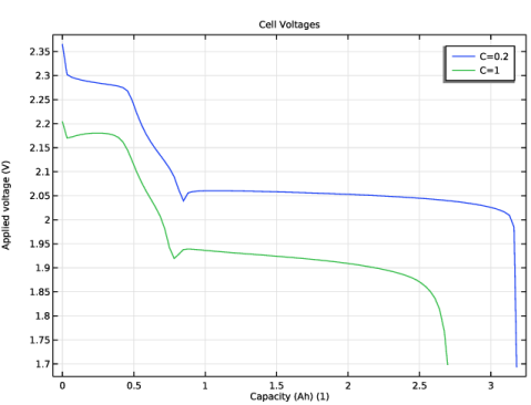
From the list, choose Galvanostatic.
|
|
5
|
|
6
|
|
7
|
|
1
|
In the Model Builder window, under Component 1 (comp1) > Definitions click Load Cycle Probe (tcd_lc1_volt).
|
|
2
|
|
3
|
|
1
|
|
3
|
|
4
|
|
1
|
In the Model Builder window, under Component 1 (comp1) > Tertiary Current Distribution, Nernst–Planck (tcd) click Initial Values 1.
|
|
2
|
|
3
|
|
4
|
|
5
|
|
6
|
|
7
|
|
8
|
|
9
|
|
10
|
|
1
|
In the Model Builder window, under Component 1 (comp1) right-click Mesh 1 and choose Edit Physics-Induced Sequence.
|
|
1
|
|
2
|
|
3
|
|
5
|
|
6
|
Locate the Element Size Parameters section.
|
|
7
|
|
1
|
|
2
|
|
3
|
Click
|
|
1
|
|
2
|
|
3
|
|
4
|
|
5
|
|
1
|
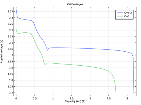
In the Model Builder window, under Results click Boundary Electrode Potential with Respect to Ground (tcd).
|
|
2
|
|
1
|
|
2
|
|
3
|
|
4
|
|
5
|
|
6
|
|
7
|
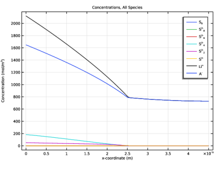
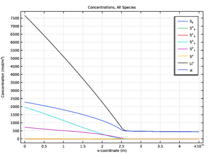
|
1
|
|
2
|
|
3
|
|
4
|
|
1
|
|
2
|
|
3
|
|
4
|
|
5
|
|
6
|
|
7
|
|
8
|
|
1
|
|
2
|
|
3
|
|
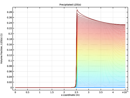
1
|
|
2
|
|
3
|
|
4
|
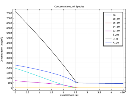
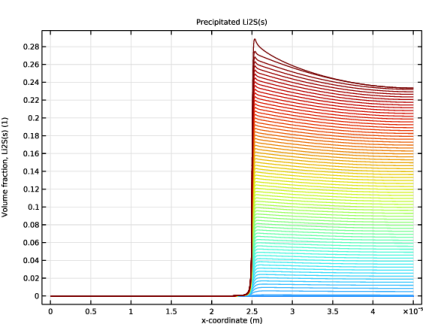
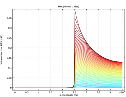
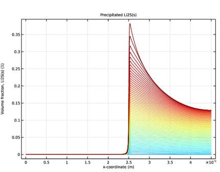
Click Replace Expression in the upper-right corner of the y-Axis Data section. From the menu, choose Component 1 (comp1) > Definitions > Variables > eps_Li2S_s - Volume fraction, Li2S(s) - 1.
|
|
5
|
|
6
|
|
7
|
Click to expand the Legends section. Find the Prefix and suffix subsection. In the Prefix text field, type Li<sub>2</sub>S(s).
|
|
8
|
|
1
|
|
2
|
|
3
|
|
4
|
|
5
|
|
6
|
|
7
|
|
8
|