| 
|
|
|
|
|
1
|
|
2
|
In the Application Libraries window, select Battery Design Module > Lithium-Ion Batteries, Performance > lib_base_model_1d in the tree.
|
|
3
|
Click
|
|
1
|
|
2
|
|
1
|
|
2
|
|
3
|
|
4
|
Browse to the model’s Application Libraries folder and double-click the file lib_power_losses_parameters.txt.
|
|
1
|
In the Model Builder window, expand the Component 1 (comp1) > Lithium-Ion Battery (liion) node, then click Load Cycle 1.
|
|
2
|
|
3
|
Select the Use elapsed time only checkbox.
|
|
1
|
|
2
|
|
1
|
|
2
|
|
3
|
|
4
|
|
5
|
|
1
|
|
2
|
|
3
|
|
1
|
|
2
|
|
3
|
|
1
|
In the Model Builder window, expand the Component 1 (comp1) > Lithium-Ion Battery (liion) > Porous Electrode - Negative node, then click Particle Intercalation 1.
|
|
2
|
|
3
|
|
4
|
Click to expand the Heat of Mixing and Power Losses section. Select the Define particle-resolved heat of mixing and power losses checkbox.
|
|
1
|
In the Model Builder window, expand the Porous Electrode - Positive node, then click Particle Intercalation 1.
|
|
2
|
|
3
|
From the Particle material list, choose NMC 111, LiNi0.33Mn0.33Co0.33O2 (Positive, Li-ion Battery) (mat3).
|
|
4
|
Locate the Heat of Mixing and Power Losses section. Select the Define particle-resolved heat of mixing and power losses checkbox.
|
|
1
|
|
2
|
|
3
|
|
4
|
|
1
|
|
2
|
|
3
|
Click
|
|
1
|
|
2
|
|
3
|
|
4
|
|
5
|
|
1
|
|
2
|
|
3
|
|
4
|
|
1
|
|
2
|
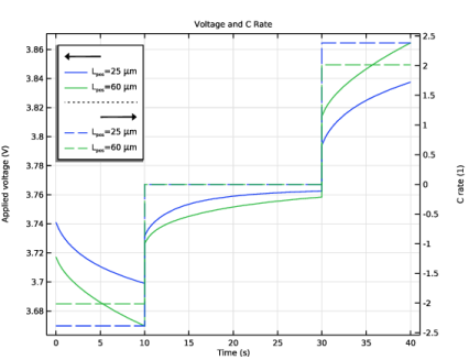
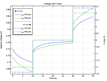
In the Settings window for Global, click Replace Expression in the upper-right corner of the y-Axis Data section. From the menu, choose Component 1 (comp1) > Lithium-Ion Battery > Load Cycle 1 > liion.lc1.E_app - Applied voltage - V.
|
|
3
|
|
4
|
|
5
|
|
1
|
|
2
|
In the Settings window for Global, click Replace Expression in the upper-right corner of the y-Axis Data section. From the menu, choose Component 1 (comp1) > Lithium-Ion Battery > Load Cycle 1 > liion.lc1.C_app - C rate - 1.
|
|
3
|
|
4
|
|
5
|
|
6
|
|
7
|
|
1
|
|
2
|
|
3
|
Select the Two y-axes checkbox.
|
|
4
|
|
5
|
|
6
|
|
1
|
|
2
|
|
3
|
|
4
|
|
5
|
|
6
|
|
7
|
|
8
|
|
9
|
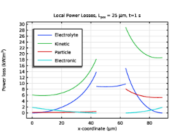
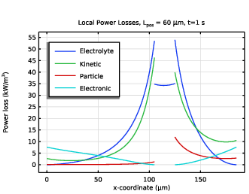
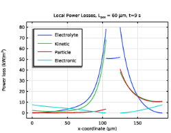
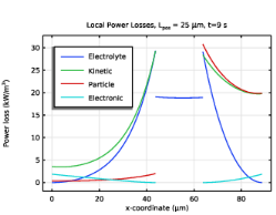
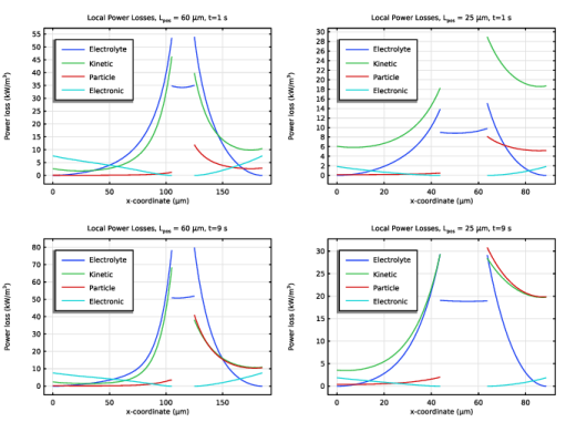
In the Title text area, type Local Power Losses, L<sub>pos</sub> = eval(L_pos*1e6) \mu m, t=eval(t) s.
|
|
1
|
|
2
|
|
3
|
|
4
|
Click Replace Expression in the upper-right corner of the y-Axis Data section. From the menu, choose Component 1 (comp1) > Lithium-Ion Battery > Power losses > liion.p_loss_l - Electrolyte transport power loss - W/m³.
|
|
5
|
|
6
|
|
7
|
|
8
|
|
9
|
|
10
|
|
11
|
|
12
|
Select the Description checkbox.
|
|
13
|
|
1
|
|
2
|
In the Settings window for Line Graph, click Replace Expression in the upper-right corner of the y-Axis Data section. From the menu, choose Component 1 (comp1) > Lithium-Ion Battery > Power losses > liion.p_loss_act - Kinetic activation power loss - W/m³.
|
|
3
|
|
4
|
|
1
|
|
2
|
In the Settings window for Line Graph, click Replace Expression in the upper-right corner of the y-Axis Data section. From the menu, choose Component 1 (comp1) > Lithium-Ion Battery > Power losses > liion.p_loss_inter - Particle intercalation transport power loss - W/m³.
|
|
3
|
|
4
|
|
1
|
|
2
|
In the Settings window for Line Graph, click Replace Expression in the upper-right corner of the y-Axis Data section. From the menu, choose Component 1 (comp1) > Lithium-Ion Battery > Power losses > liion.p_loss_s - Electron conduction power loss - W/m³.
|
|
3
|
|
4
|
|
1
|
|
2
|
|
3
|
|
4
|
|
5
|
|
6
|
|
7
|
|
8
|
|
9
|
|
10
|
|
11
|
|
1
|
|
2
|
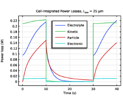
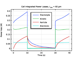
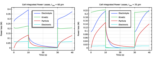
In the Settings window for 1D Plot Group, type Cell-Integrated Power Losses in the Label text field.
|
|
3
|
|
4
|
|
5
|
|
6
|
|
7
|
|
1
|
|
2
|
In the Settings window for Global, click Replace Expression in the upper-right corner of the y-Axis Data section. From the menu, choose Component 1 (comp1) > Lithium-Ion Battery > Power losses > Cell integrated > liion.P_loss_l - Electrolyte transport power loss - W.
|
|
3
|
Locate the y-Axis Data section. In the table, enter the following settings:
|
|
4
|
|
1
|
|
2
|
In the Settings window for Global, click Replace Expression in the upper-right corner of the y-Axis Data section. From the menu, choose Component 1 (comp1) > Lithium-Ion Battery > Power losses > Cell integrated > liion.P_loss_act - Kinetic activation power loss - W.
|
|
3
|
Locate the y-Axis Data section. In the table, enter the following settings:
|
|
4
|
|
1
|
|
2
|
In the Settings window for Global, click Replace Expression in the upper-right corner of the y-Axis Data section. From the menu, choose Component 1 (comp1) > Lithium-Ion Battery > Power losses > Cell integrated > liion.P_loss_inter - Particle intercalation transport power loss - W.
|
|
3
|
Locate the y-Axis Data section. In the table, enter the following settings:
|
|
4
|
|
1
|
|
2
|
In the Settings window for Global, click Replace Expression in the upper-right corner of the y-Axis Data section. From the menu, choose Component 1 (comp1) > Lithium-Ion Battery > Power losses > Cell integrated > liion.P_loss_s - Electron conduction power loss - W.
|
|
3
|
|
4
|
Locate the y-Axis Data section. In the table, enter the following settings:
|
|
1
|
|
2
|
|
3
|
|
4
|
|
5
|
|
6
|
|
1
|
|
2
|
|
3
|
|
4
|
|
5
|
|
6
|
|
7
|
|
1
|
|
2
|
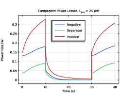
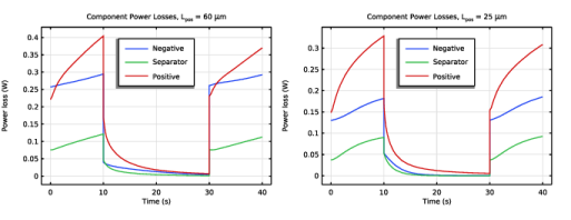
In the Settings window for Global, click Replace Expression in the upper-right corner of the y-Axis Data section. From the menu, choose Component 1 (comp1) > Lithium-Ion Battery > Power losses > Feature-node integrated > liion.pce1.P_loss - Total power loss - W.
|
|
3
|
|
4
|
|
1
|
|
2
|
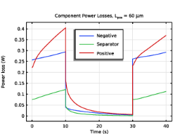
In the Settings window for Global, click Replace Expression in the upper-right corner of the y-Axis Data section. From the menu, choose Component 1 (comp1) > Lithium-Ion Battery > Power losses > Feature-node integrated > liion.sep1.P_loss - Total power loss - W.
|
|
3
|
|
4
|
|
6
|
|
1
|
|
2
|
In the Settings window for Global, click Replace Expression in the upper-right corner of the y-Axis Data section. From the menu, choose Component 1 (comp1) > Lithium-Ion Battery > Power losses > Feature-node integrated > liion.pce2.P_loss - Total power loss - W.
|
|
3
|
|
5
|
Select the Show legends checkbox.
|
|
1
|
|
2
|
|
3
|
|
4
|
|
5
|
|
6
|
|
1
|
|
2
|
|
3
|
|
4
|
|
1
|
|
2
|
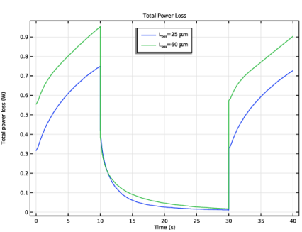
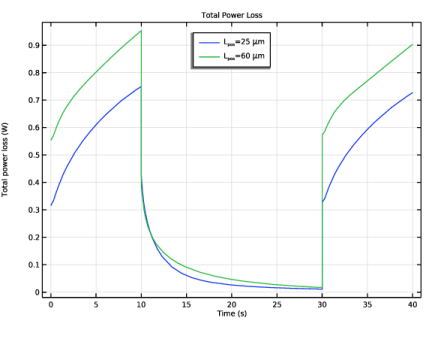
In the Settings window for Global, click Replace Expression in the upper-right corner of the y-Axis Data section. From the menu, choose Component 1 (comp1) > Lithium-Ion Battery > Power losses > Cell integrated > liion.P_loss - Total power loss - W.
|
|
3
|
|
4
|
|
1
|
|
2
|
|
3
|
|
4
|