PDF

Lithium-Ion Battery with Single-Ion Conducting Solid Electrolyte
Introduction
In solid-state lithium-ion batteries the electrolyte is a solid-state ionic conductor. The absence of a liquid electrolyte — and hence the lack of need for a liquid container and separator — implies a larger freedom of design. Additionally, solid electrolytes offer certain advantages such as no electrolyte leakage and improved thermal stability. The risk of the formation of lithium metal dendrites, which short-circuit the battery cell, is also reduced when using a solid electrolyte.
Single-ion conducting electrolytes are typically synthesized by the immobilization of the counter-ion within an inorganic particle or a polymer backbone. These single-ion conductors have a transport number close to 1 and negligible concentration gradients with regards to the charge-carrying ions.
This tutorial models a lithium-ion battery with a single-ion conducting solid electrolyte. The geometry is in one-dimension and the model is isothermal. The behavior at various discharge currents and solid electrolyte conductivities is analyzed. Additionally, a lithium-ion battery with a binary liquid electrolyte is simulated and its performance is compared to the solid state battery.
Model Definition
The model is set up for a graphite/LCO battery with a solid electrolyte. The electrode materials are available from the Battery material library and mainly default settings are selected. The conductivity of the solid electrolyte is set using a user-defined parameter.
The model is set up using the Lithium-Ion Battery, Single-Ion Conductor interface. This adds a Lithium-ion Battery interface with the charge balance model set to Single-Ion Conductor, that is typically applicable to solid electrolytes. In a single-ion conducting electrolyte it is assumed that only one ion is allowed to move, whereas the counter-ion is fixed. The assumption of electroneutrality and a constant concentration of the immobilized ions results in a constant concentration for the mobile lithium ions in the electrolyte. The Single-Ion Conductor charge balance model, thereby, solves for the electrolyte potential by assuming that all charge in the electrolyte phase is carried by the positive lithium ions only, so that the concentration of lithium ions in the electrolyte can be assumed to be constant. The electrolyte concentration is hence not solved for as a dependent variable.
The interface, with the single-ion conductor charge balance model, accounts for the following:
This tutorial, as defined in the Modeling Instructions section below, consists of two parts. The first part simulates the discharge of a lithium-ion battery with a solid electrolyte, using the Single-Ion Conductor charge balance model, for a range of discharge currents and electrolyte conductivities. In the second part of the model, a lithium-ion battery with a binary liquid electrolyte is simulated and its performance is compared to that of the solid-state battery for different discharge currents. Note that the model file available in Application Libraries contains the first part only.
The second part of the tutorial includes a binary liquid electrolyte, 1M LiPF6 in 3:7 EC:EMC (available from the Battery material library). In this case, the Binary 1:1 Liquid Electrolyte charge balance model is used along with concentration dependent electrolyte conductivity. Note that the Binary 1:1 Liquid Electrolyte charge balance model additionally accounts for material transport in the electrolyte (that is, electrolyte concentration is solved for as a dependent variable), allowing for the introduction of the effects of concentration on ionic conductivity and concentration overpotential.
Study settings
The Time Dependent with Initialization study is used in this model. This study solves for a Current Distribution Initialization study step followed by a Time Dependent study step. A stop condition is used in the Time Dependent study step to stop the solver when the cell voltage reaches 2.7 V. The SOC and Initial Charge Distribution feature is used to define the initial charge inventory in the cell.
The study corresponding to the first part of the tutorial (solid electrolyte battery) sets up an Auxiliary sweep over-discharge C-rates (1C, 2C, and 4C) and solid electrolyte conductivities (0.02 S/m, 0.05 S/m, 0.5 S/m, and 1 S/m). The study corresponding to the second part of the tutorial (binary liquid electrolyte battery) sets up an Auxiliary sweep over-discharge C-rates only.
Results and Discussion
Figure 1 and Figure 2 show the cell voltage profiles at electrolyte conductivity of 0.02 S/m and 1 S/m, respectively. The battery performance is higher at higher values of electrolyte conductivity. This is as expected, since the internal losses in the battery increase as the conductivity of the solid electrolyte is decreased.
Figure 1: Cell voltage profiles at electrolyte conductivity of 0.02 S/m.
Figure 2: Cell voltage profiles at electrolyte conductivity of 1 S/m.
Figure 3 and Figure 4 show the 1C discharge voltage profiles for different values of electrolyte conductivity ranging from 0.02 S/m to 1 S/m. The 4C discharge profiles (Figure 4) clearly indicate decreased battery performance for lower values of electrolyte conductivity.
Figure 3: Cell voltage profiles at 1C for different values of electrolyte conductivity.
Figure 4: Cell voltage profiles at 4C for different values of electrolyte conductivity.
Figure 5 and Figure 6 show the electrolyte potential drop across the cell at discharge rate of 1C, for two different values of electrolyte conductivity. The voltage drop in the electrolyte is higher for lower values of electrolyte conductivity, as seen in Figure 5.
Figure 5: Electrolyte potential drop at 1C and an electrolyte conductivity of 0.02 S/m.
Figure 6: Electrolyte potential drop at 1C and an electrolyte conductivity of 1 S/m.
Figure 7 shows a comparison of the cell voltage profiles for a battery with a solid electrolyte to that containing a binary liquid electrolyte. The electrolyte conductivity in the case of the solid electrolyte battery (modeled using the Single-Ion Conductor charge balance model) is considered to be 1 S/m. On the other hand, concentration dependent electrolyte conductivity is considered for the liquid electrolyte (1M LiPF6 in 3:7 EC:EMC) used in the binary liquid electrolyte battery (modeled using the Binary 1:1 Liquid Electrolyte charge balance model). Since the conductivity of the binary liquid electrolyte at initial electrolyte concentration of 1M is nearly 1 S/m, the initial voltage at each discharge rate would be identical for both the solid and liquid electrolyte cases. The cell profiles would begin to differ at later discharge times, as the local conductivity for the binary liquid electrolyte battery begins to change due to concentration gradients. Additionally, the concentration gradients would be higher at higher discharge rates, indicating a greater difference at higher discharge rates, as seen in Figure 7.
The comparison plot also indicates that for a battery with a binary liquid electrolyte, one can use the Single-Ion Conductor charge balance model for simulating low discharge/charge scenarios where significant concentration gradients would not be expected. In such cases of low discharge/charge scenarios, the Single-Ion Conductor charge balance model would provide reduced computational loads, since the electrolyte concentration is not solved for as a degree of freedom, without significant loss in accuracy (particularly useful in the case of large models).
Figure 7: A comparison of the cell voltage profiles for the single-ion conductor (at electrolyte conductivity of 1 S/m) and binary liquid electrolyte charge balance models.
References
1. N. Wolff, F. Roder, and U. Krewer, “Model Based Assessment of Performance of Lithium-Ion Batteries Using Single-Ion Conducting Electrolytes,” Electrochimica Acta, vol. 284, pp. 639–646, 2018.
2. S.D. Fabre, D. Guy-Bouyssou, P. Bouillon, F. Le Cras, and C. Delacourt, “Charge/Discharge Simulation of an All-Solid-State Thin-Film Battery Using a One-Dimensional Model,” J. Electrochemical Society, vol. 159, pp. A104–A115, 2012.
Application Library path: Battery_Design_Module/Lithium-Ion_Batteries,_Performance/li_battery_solid_electrolyte
Modeling Instructions
This tutorial consists of two parts. The first part simulates the discharge of a lithium-ion battery with a solid electrolyte, by using the Single-Ion Conductor charge balance model, for a range of discharge currents and electrolyte conductivities. The second part compares the performance of a lithium-ion battery containing a solid electrolyte to that containing a binary liquid electrolyte for different discharge currents. Note that the tutorial available in Application Libraries contains the first part only.
From the File menu, choose New.
New
In the New window, click  Model Wizard.
Model Wizard
1
In the Model Wizard window, click  1D.
2
In the Select Physics tree, select Electrochemistry > Batteries > Lithium-Ion Battery, Single-Ion Conductor (liion).
3
Click Add.
4
Click  Study.
5
In the Select Study tree, select Preset Studies for Selected Physics Interfaces > Time Dependent with Initialization.
(The Time Dependent with Initialization study will perform a time-dependent simulation, using an initialization study step to calculate the initial potentials in the cell.)
6
Global Definitions
Parameters 1
Load the parameters for this model from a text file.
1
In the Model Builder window, under Global Definitions click Parameters 1.
2
In the Settings window for Parameters, locate the Parameters section.
3
Click  Load from File.
4
Geometry 1
The geometry contains three domains. Create the geometry by specifying the lengths of the domains.
Interval 1 (i1)
1
In the Model Builder window, under Component 1 (comp1) right-click Geometry 1 and choose Interval.
2
In the Settings window for Interval, locate the Interval section.
3
From the Specify list, choose Interval lengths.
4
5
Click  Build Selected.
Add Material
The negative and positive electrode properties are specified using material properties (corresponding materials imported from the Battery material library), whereas the solid electrolyte properties are specified using user-defined parameters. The model has a graphite negative electrode and a LCO positive electrode.
1
In the Home toolbar, click  Add Material to open the Add Material window.
2
Go to the Add Material window.
3
In the tree, select Battery > Electrodes > Graphite, LixC6 MCMB (Negative, Li-ion Battery).
4
Click the Add to Component button in the window toolbar.
5
In the tree, select Battery > Electrodes > LCO, LiCoO2 (Positive, Li-ion Battery).
6
Click the Add to Component button in the window toolbar.
7
In the Home toolbar, click  Add Material to close the Add Material window.
Materials
Graphite, LixC6 MCMB (Negative, Li-ion Battery) (mat1)
1
In the Settings window for Material, locate the Geometric Entity Selection section.
2
Click  Clear Selection.
3
LCO, LiCoO2 (Positive, Li-ion Battery) (mat2)
1
In the Model Builder window, click LCO, LiCoO2 (Positive, Li-ion Battery) (mat2).
2
Definitions
Integration 1 (intop1)
Define boundary integration variables in order to access the cell voltage at the end terminals during computation and postprocessing.
1
In the Definitions toolbar, click  Nonlocal Couplings and choose Integration.
2
In the Settings window for Integration, type PositiveCC in the Operator name text field.
3
Locate the Source Selection section. From the Geometric entity level list, choose Boundary.
4
Integration 2 (PositiveCC2)
1
Right-click Integration 1 (PositiveCC) and choose Duplicate.
2
In the Settings window for Integration, type NegativeCC in the Operator name text field.
3
Locate the Source Selection section. Click  Clear Selection.
4
Lithium-Ion Battery (liion)
Set up the physics in the model. Use the SOC and Initial Charge Distribution node in order to calculate the initial charge distribution in the cell.
Separator 1
1
In the Model Builder window, under Component 1 (comp1) > Lithium-Ion Battery (liion) click Separator 1.
2
In the Settings window for Separator, locate the Electrolyte Properties section.
3
From the σl list, choose User defined. In the associated text field, type sigmal.
Porous Electrode 1
1
In the Physics toolbar, click  Domains and choose Porous Electrode.
2
3
In the Settings window for Porous Electrode, locate the Electrolyte Properties section.
4
From the σl list, choose User defined. In the associated text field, type sigmal.
5
Locate the Electrode Properties section. In the σs text field, type sigmas_neg.
6
Locate the Porous Matrix Properties section. In the εs text field, type epss_neg.
Particle Intercalation 1
1
In the Model Builder window, click Particle Intercalation 1.
2
In the Settings window for Particle Intercalation, locate the Particle Transport Properties section.
3
In the rp text field, type rp.
Porous Electrode Reaction 1
1
In the Model Builder window, click Porous Electrode Reaction 1.
2
In the Settings window for Porous Electrode Reaction, locate the Electrode Kinetics section.
3
In the i0,ref(T) text field, type i0ref_neg.
Porous Electrode 2
1
In the Physics toolbar, click  Domains and choose Porous Electrode.
2
3
In the Settings window for Porous Electrode, locate the Electrolyte Properties section.
4
From the σl list, choose User defined. In the associated text field, type sigmal.
5
Locate the Electrode Properties section. In the σs text field, type sigmas_pos.
6
Locate the Porous Matrix Properties section. In the εs text field, type epss_pos.
Particle Intercalation 1
1
In the Model Builder window, click Particle Intercalation 1.
2
In the Settings window for Particle Intercalation, locate the Particle Transport Properties section.
3
In the rp text field, type rp.
Porous Electrode Reaction 1
1
In the Model Builder window, click Porous Electrode Reaction 1.
2
In the Settings window for Porous Electrode Reaction, locate the Electrode Kinetics section.
3
In the i0,ref(T) text field, type i0ref_pos.
4
In the Model Builder window, click Lithium-Ion Battery (liion).
5
In the Settings window for Lithium-Ion Battery, locate the Cell Settings section.
6
Select the Define cell state of charge (SOC) and initial charge inventory checkbox.
SOC and Initial Charge Distribution 1
1
In the Model Builder window, under Component 1 (comp1) > Lithium-Ion Battery (liion) click SOC and Initial Charge Distribution 1.
2
In the Settings window for SOC and Initial Charge Distribution, locate the Initial Cell Charge Distribution section.
3
In the SOC0 text field, type SOC_0.
4
Clear the Add formation loss checkbox.
Negative Electrode Domain Selection 1
Select which model domains that represent the negative and positive electrode, respectively.
1
In the Model Builder window, click Negative Electrode Domain Selection 1.
2
Positive Electrode Domain Selection 1
1
In the Model Builder window, click Positive Electrode Domain Selection 1.
2
Electric Ground 1
Finish by setting the boundary conditions. Ground is set as reference at the leftmost boundary, the negative electrode current collector. A current is applied at the rightmost boundary, the positive electrode current collector. Note that 1C current is available from the SOC and Initial Charge Distribution node.
1
In the Physics toolbar, click  Boundaries and choose Electric Ground.
2
Electrode Current 1
1
In the Physics toolbar, click  Boundaries and choose Electrode Current.
2
3
In the Settings window for Electrode Current, locate the Electrode Current section.
4
From the list, choose C-rate multiple.
5
In the Crate text field, type -C_rate.
6
In the ϕs,bnd,init text field, type 4[V].
Study 1
Modify the Time Dependent with Initialization study, to perform an Auxiliary sweep over discharge C-rates and solid electrolyte conductivities.
Step 2: Time Dependent
1
In the Model Builder window, under Study 1 click Step 2: Time Dependent.
2
In the Settings window for Time Dependent, locate the Study Settings section.
3
In the Output times text field, type 0 4000.
4
Click to expand the Study Extensions section. Select the Auxiliary sweep checkbox.
5
From the Sweep type list, choose All combinations.
6
7
8
9
Solution 1 (sol1)
1
In the Study toolbar, click  Show Default Solver.
Store the actual steps taken by the solver to make sure to capture any sudden steep voltage changes.
2
In the Model Builder window, expand the Solution 1 (sol1) node, then click Time-Dependent Solver 1.
3
In the Settings window for Time-Dependent Solver, locate the General section.
4
From the Times to store list, choose Steps taken by solver.
5
Right-click Study 1 > Solver Configurations > Solution 1 (sol1) > Time-Dependent Solver 1 and choose Stop Condition.
6
In the Settings window for Stop Condition, locate the Stop Expressions section.
7
8
9
Locate the Output at Stop section. From the Add solution list, choose Step before stop.
10
Clear the Add information checkbox.
11
In the Model Builder window, click Study 1.
12
In the Settings window for Study, locate the Study Settings section.
13
Clear the Generate default plots checkbox.
14
In the Study toolbar, click  Compute.
Results
Reproduce the plots in the model documentation, starting with the cell voltage profiles at electrolyte conductivity of 0.02S/m (Figure 1).
Cell Voltage: sigmal = 0.02 S/m
1
In the Results toolbar, click  1D Plot Group.
2
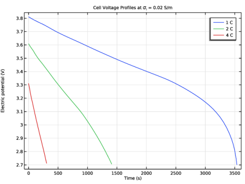
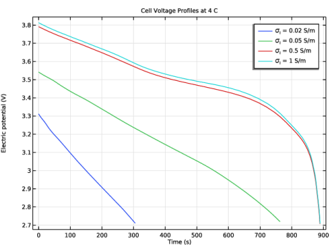
In the Settings window for 1D Plot Group, type Cell Voltage: sigmal = 0.02 S/m in the Label text field.
3
Locate the Data section. From the Parameter selection (sigmal) list, choose First.
Point Graph 1
1
Right-click Cell Voltage: sigmal = 0.02 S/m and choose Point Graph.
2
3
In the Settings window for Point Graph, click Replace Expression in the upper-right corner of the y-Axis Data section. From the menu, choose Component 1 (comp1) > Lithium-Ion Battery > phis - Electric potential - V.
4
Click to expand the Legends section. Select the Show legends checkbox.
5
From the Legends list, choose Evaluated.
6
In the Legend text field, type eval(C_rate) C.
Cell Voltage: sigmal = 0.02 S/m
1
In the Model Builder window, click Cell Voltage: sigmal = 0.02 S/m.
2
In the Settings window for 1D Plot Group, click to expand the Title section.
3
From the Title type list, choose Manual.
4
In the Title text area, type Cell Voltage Profiles at \sigma<sub>l</sub> = 0.02 S/m.
5
In the Cell Voltage: sigmal = 0.02 S/m toolbar, click  Plot.
Now, duplicate the previous figure to create a plot of the cell voltage profiles at electrolyte conductivity of 1S/m (Figure 2).
Cell Voltage: sigmal = 1 S/m
1
Right-click Cell Voltage: sigmal = 0.02 S/m and choose Duplicate.
2
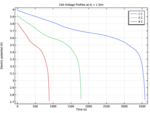
In the Settings window for 1D Plot Group, type Cell Voltage: sigmal = 1 S/m in the Label text field.
3
Locate the Data section. From the Parameter selection (sigmal) list, choose Last.
4
Locate the Title section. In the Title text area, type Cell Voltage Profiles at \sigma<sub>l</sub> = 1 S/m.
5
In the Cell Voltage: sigmal = 1 S/m toolbar, click  Plot.
Cell Voltage: 1 C
Next, create cell voltage profiles plots at 1 C (Figure 3) and 4 C (Figure 4), respectively, for different value of electrolyte conductivity.
1
In the Results toolbar, click  1D Plot Group.
2
In the Settings window for 1D Plot Group, type Cell Voltage: 1 C in the Label text field.
3
Locate the Data section. From the Parameter selection (C_rate) list, choose First.
Point Graph 1
1
Right-click Cell Voltage: 1 C and choose Point Graph.
2
3
In the Settings window for Point Graph, click Replace Expression in the upper-right corner of the y-Axis Data section. From the menu, choose Component 1 (comp1) > Lithium-Ion Battery > phis - Electric potential - V.
4
Locate the Legends section. Select the Show legends checkbox.
5
From the Legends list, choose Evaluated.
6
In the Legend text field, type \sigma<sub>l</sub> = eval(sigmal) S/m.
Cell Voltage: 1 C
1
In the Model Builder window, click Cell Voltage: 1 C.
2
In the Settings window for 1D Plot Group, locate the Title section.
3
From the Title type list, choose Manual.
4
In the Title text area, type Cell Voltage Profiles at 1 C.
5
In the Cell Voltage: 1 C toolbar, click  Plot.
Cell Voltage: 4 C
1
Right-click Cell Voltage: 1 C and choose Duplicate.
2
In the Settings window for 1D Plot Group, type Cell Voltage: 4 C in the Label text field.
3
Locate the Data section. From the Parameter selection (C_rate) list, choose Last.
4
Locate the Title section. In the Title text area, type Cell Voltage Profiles at 4 C.
5
In the Cell Voltage: 4 C toolbar, click  Plot.
Electrolyte Potential Drop: 1 C and sigmal = 0.02 S/m
Next, create plots depicting the electrolyte potential drop at 1C, for two values of electrolyte conductivity. Figure 5 and Figure 6 correspond, respectively, to electrolyte conductivity values of 0.02S/m and 1S/m.
1
In the Results toolbar, click  1D Plot Group.
2
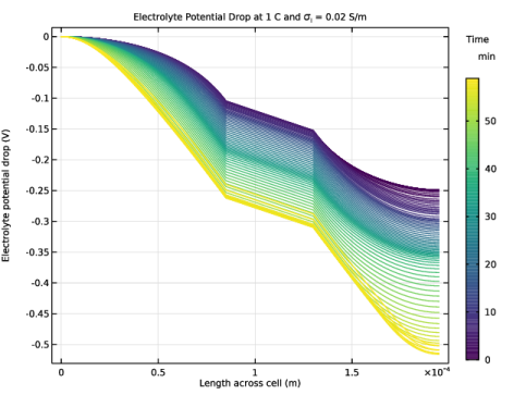
In the Settings window for 1D Plot Group, type Electrolyte Potential Drop: 1 C and sigmal = 0.02 S/m in the Label text field.
3
Locate the Data section. From the Parameter selection (C_rate) list, choose First.
4
From the Parameter selection (sigmal) list, choose First.
Line Graph 1
1
Right-click Electrolyte Potential Drop: 1 C and sigmal = 0.02 S/m and choose Line Graph.
2
In the Settings window for Line Graph, locate the Selection section.
3
From the Selection list, choose All domains.
4
Locate the y-Axis Data section. In the Expression text field, type phil-NegativeCC(phil).
Color Expression 1
1
In the Electrolyte Potential Drop: 1 C and sigmal = 0.02 S/m toolbar, click  Color Expression.
2
In the Settings window for Color Expression, locate the Expression section.
3
In the Expression text field, type t.
4
From the Unit list, choose min.
5
Locate the Coloring and Style section. From the Color table list, choose Viridis.
6
Click to expand the Title section.
Electrolyte Potential Drop: 1 C and sigmal = 0.02 S/m
1
In the Model Builder window, under Results click Electrolyte Potential Drop: 1 C and sigmal = 0.02 S/m.
2
In the Settings window for 1D Plot Group, locate the Title section.
3
From the Title type list, choose Manual.
4
In the Title text area, type Electrolyte Potential Drop at 1 C and \sigma<sub>l</sub> = 0.02 S/m.
5
Locate the Plot Settings section.
6
Select the x-axis label checkbox. In the associated text field, type Length across cell (m).
7
Select the y-axis label checkbox. In the associated text field, type Electrolyte potential drop (V).
8
Locate the Color Legend section. Select the Show titles checkbox.
9
Select the Show units checkbox.
Color Expression 1
1
In the Model Builder window, under Results > Electrolyte Potential Drop: 1 C and sigmal = 0.02 S/m > Line Graph 1 click Color Expression 1.
2
In the Settings window for Color Expression, locate the Coloring and Style section.
3
In the Color legend title text field, type Time.
Electrolyte Potential Drop: 1 C and sigmal = 0.02 S/m
1
In the Model Builder window, under Results click Electrolyte Potential Drop: 1 C and sigmal = 0.02 S/m.
2
In the Electrolyte Potential Drop: 1 C and sigmal = 0.02 S/m toolbar, click  Plot.
Electrolyte Potential Drop: 1 C and sigmal = 1 S/m
1
Right-click Electrolyte Potential Drop: 1 C and sigmal = 0.02 S/m and choose Duplicate.
2
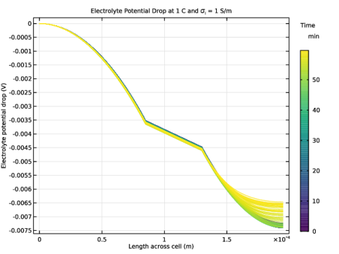
In the Settings window for 1D Plot Group, type Electrolyte Potential Drop: 1 C and sigmal = 1 S/m in the Label text field.
3
Locate the Data section. From the Parameter selection (sigmal) list, choose Last.
4
Locate the Title section. In the Title text area, type Electrolyte Potential Drop at 1 C and \sigma<sub>l</sub> = 1 S/m.
5
In the Electrolyte Potential Drop: 1 C and sigmal = 1 S/m toolbar, click  Plot.
Materials
The first part of the tutorial is now complete. In the second part, the performance of a lithium-ion battery containing a solid electrolyte is compared to that containing a binary liquid electrolyte. Now let us proceed to modify the model setup for a binary liquid electrolyte. Start by adding an electrolyte material and subsequently modifying the physics settings.
Add Material
1
In the Materials toolbar, click  Add Material to open the Add Material window.
2
Go to the Add Material window.
3
In the tree, select Battery > Electrolytes > LiPF6 in 3:7 EC:EMC (Liquid, Li-ion Battery).
4
Click the Add to Component button in the window toolbar.
5
In the Materials toolbar, click  Add Material to close the Add Material window.
Materials
LiPF6 in 3:7 EC:EMC (Liquid, Li-ion Battery) (mat3)
Select Domain 2 only.
Lithium-Ion Battery (liion)
1
In the Model Builder window, under Component 1 (comp1) click Lithium-Ion Battery (liion).
2
In the Settings window for Lithium-Ion Battery, locate the Charge Balance Model section.
3
From the list, choose Binary 1:1 liquid electrolyte.
Separator 1
1
In the Model Builder window, under Component 1 (comp1) > Lithium-Ion Battery (liion) click Separator 1.
2
In the Settings window for Separator, locate the Electrolyte Properties section.
3
From the σl list, choose From material.
Porous Electrode 1
1
In the Model Builder window, click Porous Electrode 1.
2
In the Settings window for Porous Electrode, locate the Electrolyte Properties section.
3
From the Electrolyte material list, choose LiPF6 in 3:7 EC:EMC (Liquid, Li-ion Battery) (mat3).
4
From the σl list, choose From material.
Porous Electrode 2
1
In the Model Builder window, click Porous Electrode 2.
2
In the Settings window for Porous Electrode, locate the Electrolyte Properties section.
3
From the Electrolyte material list, choose LiPF6 in 3:7 EC:EMC (Liquid, Li-ion Battery) (mat3).
4
From the σl list, choose From material.
Add Study
Add a Time Dependent with Initialization study as before, to perform an Auxiliary sweep over discharge C-rates.
1
In the Home toolbar, click  Add Study to open the Add Study window.
2
Go to the Add Study window.
3
Find the Studies subsection. In the Select Study tree, select Preset Studies for Selected Physics Interfaces > Time Dependent with Initialization.
4
Click the Add Study button in the window toolbar.
5
In the Home toolbar, click  Add Study to close the Add Study window.
Study 2
Step 2: Time Dependent
1
In the Settings window for Time Dependent, locate the Study Settings section.
2
In the Output times text field, type 0 4000.
3
Locate the Study Extensions section. Select the Auxiliary sweep checkbox.
4
5
Solution 3 (sol3)
1
In the Study toolbar, click  Show Default Solver.
2
In the Model Builder window, expand the Solution 3 (sol3) node, then click Time-Dependent Solver 1.
3
In the Settings window for Time-Dependent Solver, locate the General section.
4
From the Times to store list, choose Steps taken by solver.
5
In the Model Builder window, expand the Study 2 > Solver Configurations > Solution 3 (sol3) > Time-Dependent Solver 1 node.
6
Right-click Study 2 > Solver Configurations > Solution 3 (sol3) > Time-Dependent Solver 1 and choose Stop Condition.
7
In the Settings window for Stop Condition, locate the Stop Expressions section.
8
9
10
Locate the Output at Stop section. From the Add solution list, choose Step before stop.
11
Clear the Add information checkbox.
12
In the Model Builder window, click Study 2.
13
In the Settings window for Study, locate the Study Settings section.
14
Clear the Generate default plots checkbox.
15
In the Study toolbar, click  Compute.
Results
Cell Voltage: Single-Ion vs. Binary
Finally, create a plot that compares the cell voltage profiles for the single-ion conductor (at electrolyte conductivity of 1S/m) and binary liquid electrolyte charge balance models (Figure 7).
1
In the Results toolbar, click  1D Plot Group.
2
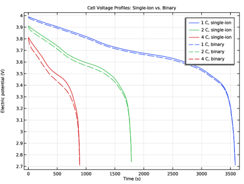
In the Settings window for 1D Plot Group, type Cell Voltage: Single-Ion vs. Binary in the Label text field.
3
Locate the Data section. From the Dataset list, choose None.
Point Graph 1
1
Right-click Cell Voltage: Single-Ion vs. Binary and choose Point Graph.
2
In the Settings window for Point Graph, locate the Data section.
3
From the Dataset list, choose Study 1/Solution 1 (sol1).
4
From the Parameter selection (sigmal) list, choose Last.
5
6
Click Replace Expression in the upper-right corner of the y-Axis Data section. From the menu, choose Component 1 (comp1) > Lithium-Ion Battery > phis - Electric potential - V.
7
Locate the x-Axis Data section. From the Axis source data list, choose Time.
8
Locate the Legends section. Select the Show legends checkbox.
9
From the Legends list, choose Evaluated.
10
In the Legend text field, type eval(C_rate) C, single-ion.
Point Graph 2
1
Right-click Point Graph 1 and choose Duplicate.
2
In the Settings window for Point Graph, locate the Data section.
3
From the Dataset list, choose Study 2/Solution 3 (sol3).
4
Click to expand the Coloring and Style section. Find the Line style subsection. From the Line list, choose Dashed.
5
From the Color list, choose Cycle (reset).
6
Locate the Legends section. In the Legend text field, type eval(C_rate) C, binary.
Cell Voltage: Single-Ion vs. Binary
1
In the Model Builder window, click Cell Voltage: Single-Ion vs. Binary.
2
In the Settings window for 1D Plot Group, locate the Title section.
3
From the Title type list, choose Manual.
4
In the Title text area, type Cell Voltage Profiles: Single-Ion vs. Binary.
5
In the Cell Voltage: Single-Ion vs. Binary toolbar, click  Plot.