PDF

Silicon–Graphite-Blended Electrode with Thermodynamic Voltage Hysteresis
Introduction
Due to its high capacity, silicon (Si) is often added to graphite in the negative electrode of lithium-ion batteries.
Silicon-graphite blended electrodes may exhibit significant thermodynamic voltage hysteresis (“path dependence”) because the equilibrium potential of the lithium–silicon intercalation reaction is dependent on the charge–discharge history of the electrode.
This example demonstrates how to add Si as an Additional Electrode Material in the Lithium-Ion Battery interface and how to define a memory variable for handling the voltage hysteresis using an additional Coefficient From PDE interface.
Model Definition
The model solves for a half cell with the following components:
Blended porous electrode with graphite (LixC6, MCMB) and silicon (LixSi), where the thickness depends on the graphite:silicon ratio; see below
Electrolyte, 1.0 M LiPF6 in EC:EMC (3:7 by weight)
The potential of the blended electrode is defined versus a reference electrode positioned at the boundary between the blended electrode and the separator.
Similar processes are accounted for as in the Lithium-Ion Battery with Multiple Intercalating Electrode Materials example, but with some exceptions: The cell has a lithium metal counter electrode instead of a negative porous electrode that provides lithium-ion flux during charge-discharge. A memory variable is used to handle the voltage hysteresis of silicon material in the blended electrode.
Electrode Material Hysteresis
The hysteresis, or path dependence, of the silicon electrode material is depicted in Figure 1. Here, the equilibrium (rest) potentials of the individual silicon and graphite materials are plotted as a function of the degree of lithiation (xGr for graphite and xSi for silicon).
Figure 1: Equilibrium potentials defined as functions of the degree of lithiation. Current-direction-dependent potential curve for silicon (upper/delithiation and lower/lithiation). Maximum and minimum lithiation degrees, xmin and xmax, correspond to the potential limits, Emin and Emax, of the blended electrode.
For silicon, the equilibrium potential exhibits hysteresis and depends on the charging direction. Graphite does not exhibit voltage hysteresis to the same degree, and in the model the potential is only dependent on the degree of lithiation.
The potential equilibrium curve for graphite is added from the Material library and used in a Porous Electrode Reaction node on the blended porous electrode domain. In the same domain, an Additional Porous Electrode Material node is also added, defining the silicon material.
The silicon potential equilibrium is defined using a user-defined expression according to (Ref. 1)
with
and
Here S is a memory variable that is set up in a Coefficient Form PDE interface in which the following equation is solved
In this way, S approaches 1 during delithiation and 1 during lithiation.
The intercalation rate is defined as
where iv denotes the volumetric electrochemical reaction current, εs the active electrode material volume fraction, and cs,max the maximum (host) capacity for lithium intercalation in mol/m3.
Electrode Balancing
The blended porous electrode thickness, Lel, depends on the areal capacity, Qel, set to 20 Ah/m2 and the chosen potential limits for 0 and 100% state of charge (SOC) using the formulation
where xmax and xmin for the materials are defined from the maximum and minimum cutoff voltages (versus the reference electrode), Emax and Emin (Figure 1)
Energy Density
The accumulated energy required for lithiation and delithiation, Elith and Edelith (Wh/m2), is computed in a Global ODEs and DAEs interface using the expressions
where Evs ref is the potential of the blended electrode versus the reference electrode during the cycle.
The energy densities, e (Wh/m3), are obtained by dividing the accumulated energies with the electrode thickness:
Note that, as a result of the electrode balancing, the electrode thickness decreases when the Si fraction increases.
The energies are also used to compute the delithiation-to-lithiation energy efficiency
Results and Discussion
The cell is simulated for a full lithiation–delithiation cycle for three different electrode blends, and two different charge–discharging C-rates. The results of the potential change with lithiation and current direction in Figure 2 demonstrate how the hysteresis becomes more prominent with a larger fraction of silicon, and at lower SOCs.
Figure 2: Blended electrode potential versus the reference electrode for three different blends for a C/10 lithiation-delithiation rate.
As shown in Figure 3, for the 1C rate, the hysteresis is more severe. For the 4% silicon-in-graphite blend it is present over the whole SOC interval.
Figure 3: Blended electrode potential versus the reference electrode for three different blends for a 1C lithiation-delithiation rate.
From the average material lithiation levels in Figure 4, it can be seen that the silicon is intercalated first when starting a charging cycle, and that graphite intercalation dominates toward the end of the charging and at the start of the discharge (at around 10 h). This is directly related to the individual equilibrium potential curves of the two materials.
Figure 4: Average material lithiation levels for a 0.1C cycle and 4% silicon-in-graphite blend.
For the higher charge-discharge rate in Figure 5, it is seen that the relative silicon utilization increases over the whole cycle.
Figure 5: Average material lithiation levels for 1C cycle and 4% silicon-in-graphite blend.
In Figure 6, the hysteresis memory variable variation for the 1C cycle is displayed. A noteworthy difference in the dynamics of the memory variable between lithiation and delithiation is seen. It also shows that the path dependence can differ along the electrode thickness. The latter phenomena is primarily observed during the delithiation.
Figure 6: Hysteresis memory variable during 1C lithiation-delithiation for 4% silicon-in-graphite blend at two electrode locations.
Figure 7 shows that the delithiation energy density increases with the silicon content regardless of C-rate.
Figure 7: Energy density for 0.1C and 1C delithiation.
In contrast, Figure 8 displays lower delithiation-to-lithiation energy efficiency with increased silicon content. This is related to the increasing hysteresis voltage differences at higher silicon levels.
Figure 8: Delithiation-to-lithiation energy efficiencies for 0.1C and 1C cycles.
Reference
1. D.R. Baker, M.W. Verbrugge, and X. Xiao, “An approach to characterize and clarify hysteresis phenomena of lithium-silicon electrodes,”J. Appl. Phys., vol. 122, p. 165105, 2017.
Application Library path: Battery_Design_Module/Lithium-Ion_Batteries,_Performance/li_battery_sigr_hysteresis
Modeling Instructions
From the File menu, choose New.
New
In the New window, click  Model Wizard.
Model Wizard
1
In the Model Wizard window, click  1D.
2
In the Select Physics tree, select Electrochemistry > Batteries > Lithium-Ion Battery (liion).
3
Click Add.
4
Click  Study.
5
In the Select Study tree, select General Studies > Time Dependent.
6
Global Definitions
Parameters 1
1
In the Model Builder window, under Global Definitions click Parameters 1.
2
In the Settings window for Parameters, locate the Parameters section.
3
Click  Load from File.
4
Some expressions will render warnings, indicating missing definitions. This is expected at this stage and will be resolved as soon as the materials are defined.
Add all materials except for LixSi (silicon) from the Material Library.
Add Material
1
In the Materials toolbar, click  Add Material to open the Add Material window.
2
Go to the Add Material window.
3
In the tree, select Battery > Electrodes > Graphite, LixC6 MCMB (Negative, Li-ion Battery).
4
Click the Add to Component button in the window toolbar.
5
In the tree, select Battery > Electrolytes > LiPF6 in 3:7 EC:EMC (Liquid, Li-ion Battery).
6
Click the Add to Component button in the window toolbar.
7
In the tree, select Battery > Electrodes > Lithium Metal, Li (Negative, Li-ion Battery).
8
Click the Add to Component button in the window toolbar.
9
In the Materials toolbar, click  Add Material to close the Add Material window.
Definitions
Import the LixSi (silicon) equilibrium potential curves using interpolation functions. Two curves are required to model the hysteresis; one for the delithiation (upper) and another for the lithiation (lower).
Interpolation - Eeq Si Upper
1
In the Definitions toolbar, click  Interpolation.
2
In the Settings window for Interpolation, type Interpolation - Eeq Si Upper in the Label text field.
3
Locate the Definition section. In the Function name text field, type Eeq_Si_upper.
4
Click  Load from File.
5
6
Locate the Interpolation and Extrapolation section. From the Extrapolation list, choose Linear.
7
Locate the Units section. In the Function table, enter the following settings:
8
Click to expand the Related Functions section. Select the Define inverse function checkbox.
9
In the Inverse function name text field, type Eeq_Si_upper_inv.
Interpolation - Eeq Si Lower
1
In the Definitions toolbar, click  Interpolation.
2
In the Settings window for Interpolation, type Interpolation - Eeq Si Lower in the Label text field.
3
Locate the Definition section. In the Function name text field, type Eeq_Si_lower.
4
Click  Load from File.
5
6
Locate the Interpolation and Extrapolation section. From the Extrapolation list, choose Linear.
7
Locate the Units section. In the Function table, enter the following settings:
8
Click to expand the Related Functions section. Select the Define inverse function checkbox.
9
In the Inverse function name text field, type Eeq_Si_lower_inv.
Geometry 1
Interval 1 (i1)
1
In the Model Builder window, under Component 1 (comp1) right-click Geometry 1 and choose Interval.
2
In the Settings window for Interval, locate the Interval section.
3
From the Specify list, choose Interval lengths.
4
5
Click  Build All Objects.
Materials
Graphite, LixC6 MCMB (Negative, Li-ion Battery) (mat1)
1
In the Model Builder window, under Component 1 (comp1) > Materials click Graphite, LixC6 MCMB (Negative, Li-ion Battery) (mat1).
2
LiPF6 in 3:7 EC:EMC (Liquid, Li-ion Battery) (mat2)
1
In the Model Builder window, click LiPF6 in 3:7 EC:EMC (Liquid, Li-ion Battery) (mat2).
2
Lithium Metal, Li (Negative, Li-ion Battery) (mat3)
1
In the Model Builder window, click Lithium Metal, Li (Negative, Li-ion Battery) (mat3).
2
In the Settings window for Material, locate the Geometric Entity Selection section.
3
From the Geometric entity level list, choose Boundary.
4
Definitions
Define integration operators at the location of the reference electrode, and the current collector of the blended electrode, to allow for local variables to be accessed globally.
Integration - Reference
1
In the Definitions toolbar, click  Nonlocal Couplings and choose Integration.
2
In the Settings window for Integration, type Integration - Reference in the Label text field.
3
In the Operator name text field, type intop_ref.
4
Locate the Source Selection section. From the Geometric entity level list, choose Boundary.
5
Integration - Current Collector
1
In the Definitions toolbar, click  Nonlocal Couplings and choose Integration.
2
In the Settings window for Integration, type Integration - Current Collector in the Label text field.
3
In the Operator name text field, type intop_cc.
4
Locate the Source Selection section. From the Geometric entity level list, choose Boundary.
5
Import variables. Some expressions will render warnings, indicating missing definitions. This is expected at this stage and will be resolved as soon as the interfaces have been fully set up. The Electrode variables include the silicon equilibrium potential and relevant definitions related to the hysteresis.
Variables - Electrode
1
In the Model Builder window, right-click Definitions and choose Variables.
2
In the Settings window for Variables, type Variables - Electrode in the Label text field.
3
Locate the Geometric Entity Selection section. From the Geometric entity level list, choose Domain.
4
5
Locate the Variables section. Click  Load from File.
6
Variables - Global
1
Right-click Definitions and choose Variables.
2
In the Settings window for Variables, type Variables - Global in the Label text field.
3
Locate the Variables section. Click  Load from File.
4
Lithium-Ion Battery (liion)
1
In the Model Builder window, under Component 1 (comp1) click Lithium-Ion Battery (liion).
2
In the Settings window for Lithium-Ion Battery, locate the Cross-Sectional Area section.
3
In the Ac text field, type A_cell.
Separator 1
1
In the Model Builder window, under Component 1 (comp1) > Lithium-Ion Battery (liion) click Separator 1.
2
In the Settings window for Separator, locate the Porous Matrix Properties section.
3
In the εl text field, type epsl_sep.
Define the graphite material properties of the blended porous electrode in a Porous Electrode node.
Porous Electrode 1 - Graphite
1
In the Physics toolbar, click  Domains and choose Porous Electrode.
2
In the Settings window for Porous Electrode, type Porous Electrode 1 - Graphite in the Label text field.
3
4
Locate the Electrolyte Properties section. From the Electrolyte material list, choose LiPF6 in 3:7 EC:EMC (Liquid, Li-ion Battery) (mat2).
5
Locate the Electrode Properties section. In the σs text field, type sigma_s.
6
Locate the Porous Matrix Properties section. In the εs text field, type epss_Gr.
7
In the εl text field, type epsl_el.
Particle Intercalation 1
1
In the Model Builder window, click Particle Intercalation 1.
2
In the Settings window for Particle Intercalation, locate the Species Settings section.
3
In the cs,init text field, type cs_Gr_init.
4
Locate the Material section. From the Particle material list, choose Graphite, LixC6 MCMB (Negative, Li-ion Battery) (mat1).
5
Locate the Particle Transport Properties section. In the rp text field, type rp_Gr.
6
Click to expand the Operational SOCs for Initial Cell Charge Distribution section. From the socmin list, choose User defined. From the socmax list, choose User defined.
Porous Electrode Reaction 1
1
In the Model Builder window, click Porous Electrode Reaction 1.
2
In the Settings window for Porous Electrode Reaction, locate the Material section.
3
From the Material list, choose Graphite, LixC6 MCMB (Negative, Li-ion Battery) (mat1).
4
Locate the Electrode Kinetics section. In the i0,ref(T) text field, type i0_ref_Gr.
Define the Silicon material properties of the blended porous electrode using an Additional Porous Electrode Material node.
Additional Porous Electrode Material 1 - Silicon
1
In the Physics toolbar, click  Domains and choose Additional Porous Electrode Material.
2
In the Settings window for Additional Porous Electrode Material, type Additional Porous Electrode Material 1 - Silicon in the Label text field.
3
4
Locate the Volume Fraction section. In the εs text field, type epss_Si.
Particle Intercalation 1
1
In the Model Builder window, click Particle Intercalation 1.
2
In the Settings window for Particle Intercalation, locate the Species Settings section.
3
In the cs,init text field, type cs_Si_init.
4
From the cs,max list, choose User defined. In the associated text field, type cs_Si_max.
5
Locate the Particle Transport Properties section. From the Species concentration transport model list, choose No spatial gradients.
6
In the rp text field, type rp_Si.
7
Click to expand the Operational SOCs for Initial Cell Charge Distribution section. From the socmin list, choose User defined. From the socmax list, choose User defined.
Porous Electrode Reaction 1
1
In the Model Builder window, click Porous Electrode Reaction 1.
2
In the Settings window for Porous Electrode Reaction, locate the Equilibrium Potential section.
3
From the Eeq list, choose User defined. In the associated text field, type Eeq_Si.
4
Locate the Electrode Kinetics section. In the i0,ref(T) text field, type i0_ref_Si.
Electrode Surface 1 - Lithium Metal
1
In the Physics toolbar, click  Boundaries and choose Electrode Surface.
2
In the Settings window for Electrode Surface, type Electrode Surface 1 - Lithium Metal in the Label text field.
3
Load Cycle 1
1
In the Physics toolbar, click  Boundaries and choose Load Cycle.
2
3
In the Settings window for Load Cycle, locate the Load Type section.
4
Current 1
1
In the Physics toolbar, click  Attributes and choose Current.
2
In the Settings window for Current, locate the Current section.
3
In the Iset text field, type -i_1C*C_rate*A_cell.
4
Locate the Continuation Conditions section. Select the User defined checkbox.
5
In the Induser text field, type -(E_vs_ref-E_switch)/1[V].
Load Cycle 1
In the Model Builder window, click Load Cycle 1.
Current 2
1
In the Physics toolbar, click  Attributes and choose Current.
2
In the Settings window for Current, locate the Current section.
3
In the Iset text field, type i_1C*C_rate*A_cell.
Load Cycle 1
1
In the Model Builder window, click Load Cycle 1.
2
In the Settings window for Load Cycle, locate the Cycling Stop Condition section.
3
4
In the Induser text field, type (E_vs_ref-E_end)/1[V].
Initial Values 1
1
In the Model Builder window, click Initial Values 1.
2
In the Settings window for Initial Values, locate the Initial Values section.
3
In the phis text field, type E_init_el.
Add a Coefficient Form PDE to compute the memory variable, S.
Add Physics
1
In the Physics toolbar, click  Add Physics to open the Add Physics window.
2
Go to the Add Physics window.
3
In the tree, select Mathematics > PDE Interfaces > Coefficient Form PDE (c).
4
Click the Add to Component 1 button in the window toolbar.
Coefficient Form PDE - Memory Variable
1
In the Settings window for Coefficient Form PDE, type Coefficient Form PDE - Memory Variable in the Label text field.
2
3
Click to expand the Dependent Variables section. In the Field name (1) text field, type S.
4
In the Dependent variables (1) table, enter the following settings:
Coefficient Form PDE 1
1
In the Model Builder window, under Component 1 (comp1) > Coefficient Form PDE - Memory Variable (c) click Coefficient Form PDE 1.
2
In the Settings window for Coefficient Form PDE, locate the Diffusion Coefficient section.
3
In the c text field, type 0.
4
Locate the Source Term section. In the f text field, type dSdt.
Initial Values 1
1
In the Model Builder window, click Initial Values 1.
2
In the Settings window for Initial Values, locate the Initial Values section.
3
In the S text field, type S_init.
Add Physics
1
Go to the Add Physics window.
2
In the tree, select Mathematics > ODE and DAE Interfaces > Global ODEs and DAEs (ge).
3
Click the Add to Component 1 button in the window toolbar.
Global ODEs and DAEs - Charge Integration
Define global Global ODEs and DAEs interfaces to compute cumulative variables.
1
In the Settings window for Global ODEs and DAEs, type Global ODEs and DAEs - Charge Integration in the Label text field.
Global Equations 1 (ODE1)
1
In the Model Builder window, under Component 1 (comp1) > Global ODEs and DAEs - Charge Integration (ge) click Global Equations 1 (ODE1).
2
In the Settings window for Global Equations, locate the Global Equations section.
3
4
Locate the Units section. Click  Define Dependent Variable Unit.
5
In the Dependent variable quantity table, enter the following settings:
6
Click  Define Source Term Unit.
7
In the Source term quantity table, enter the following settings:
Add Physics
1
Go to the Add Physics window.
2
In the tree, select Mathematics > ODE and DAE Interfaces > Global ODEs and DAEs (ge).
3
Click the Add to Component 1 button in the window toolbar.
4
In the Home toolbar, click  Add Physics to close the Add Physics window.
Global ODEs and DAEs - Energy Integration
In the Settings window for Global ODEs and DAEs, type Global ODEs and DAEs - Energy Integration in the Label text field.
Global Equations 1 (ODE2)
1
In the Model Builder window, under Component 1 (comp1) > Global ODEs and DAEs - Energy Integration (ge2) click Global Equations 1 (ODE2).
2
In the Settings window for Global Equations, locate the Global Equations section.
3
4
Locate the Units section. Click  Define Dependent Variable Unit.
5
In the Dependent variable quantity table, enter the following settings:
6
Click  Define Source Term Unit.
7
In the Source term quantity table, enter the following settings:
Study 1
Set up a parametric sweep to simulate the half cell for different C-rates and blended electrode compositions.
Parametric Sweep
1
In the Study toolbar, click  Parametric Sweep.
2
In the Settings window for Parametric Sweep, locate the Study Settings section.
3
4
5
6
7
From the Sweep type list, choose All combinations.
Step 1: Time Dependent
1
In the Model Builder window, click Step 1: Time Dependent.
2
In the Settings window for Time Dependent, locate the Study Settings section.
3
From the Time unit list, choose h.
4
In the Output times text field, type range(0,0.01/C_rate,2.1/C_rate).
5
In the Study toolbar, click  Compute.
The following steps reproduce the model figures.
Results
0.1 C Electrode Voltage vs. SOC
1
In the Model Builder window, under Results click Boundary Electrode Potential with Respect to Ground (liion).
2
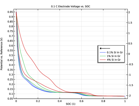
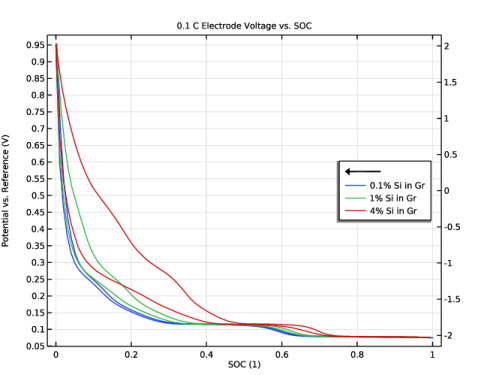
In the Settings window for 1D Plot Group, type 0.1 C Electrode Voltage vs. SOC in the Label text field.
3
Locate the Data section. From the Parameter selection (C_rate) list, choose First.
4
Click to expand the Title section. From the Title type list, choose Label.
5
Locate the Plot Settings section.
6
Select the y-axis label checkbox. In the associated text field, type Potential vs. Reference (V).
7
Select the x-axis label checkbox. In the associated text field, type SOC (1).
Global 1
1
In the Model Builder window, expand the 0.1 C Electrode Voltage vs. SOC node, then click Global 1.
2
In the Settings window for Global, click Replace Expression in the upper-right corner of the y-Axis Data section. From the menu, choose Component 1 (comp1) > Definitions > Variables > E_vs_ref - Electrode potential vs. reference - V.
3
Locate the x-Axis Data section. From the Axis source data list, choose Inner solutions.
4
From the Parameter list, choose Expression.
5
Click Replace Expression in the upper-right corner of the x-Axis Data section. From the menu, choose Component 1 (comp1) > Definitions > Variables > SOC - Electrode SOC - 1.
6
Click to expand the Legends section. Find the Include subsection. Clear the Description checkbox.
7
Find the Prefix and suffix subsection. In the Prefix text field, type eval(Si_f*100)% Si in Gr.
Global 2
In the Model Builder window, right-click Global 2 and choose Delete.
0.1 C Electrode Voltage vs. SOC
1
In the Model Builder window, under Results click 0.1 C Electrode Voltage vs. SOC.
2
In the 0.1 C Electrode Voltage vs. SOC toolbar, click  Plot.
1 C Electrode Voltage vs. SOC
1
Right-click 0.1 C Electrode Voltage vs. SOC and choose Duplicate.
2
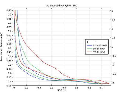
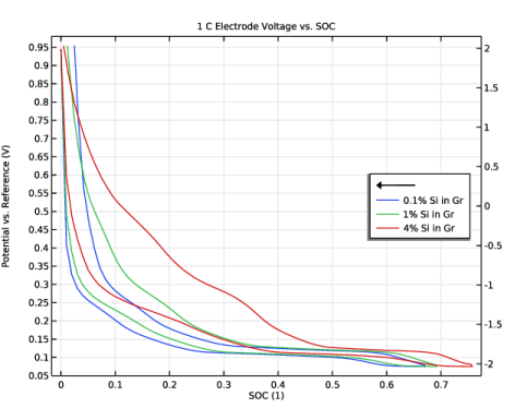
In the Settings window for 1D Plot Group, type 1 C Electrode Voltage vs. SOC in the Label text field.
3
Locate the Data section. From the Parameter selection (C_rate) list, choose Last.
4
In the 1 C Electrode Voltage vs. SOC toolbar, click  Plot.
0.1 C Average Material Lithiation Levels
1
In the Model Builder window, under Results click Average Electrode State of Charge (liion).
2
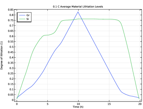
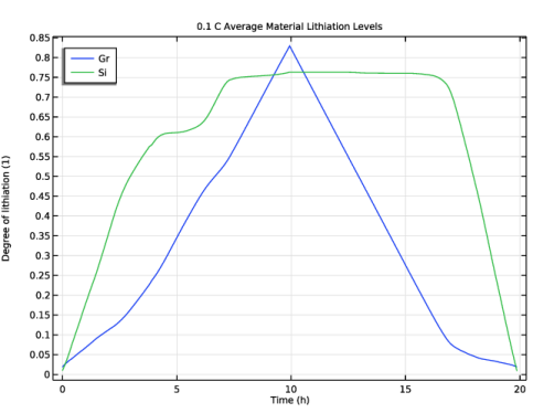
In the Settings window for 1D Plot Group, type 0.1 C Average Material Lithiation Levels in the Label text field.
3
Locate the Data section. From the Parameter selection (C_rate) list, choose First.
4
From the Parameter selection (Si_f) list, choose From list.
5
In the Parameter values (Si_f (%)) list box, select 4.
6
Locate the Title section. From the Title type list, choose Label.
7
Locate the Plot Settings section. In the y-axis label text field, type Degree of lithiation (1).
8
Locate the Legend section. From the Position list, choose Upper left.
Global 1
1
In the Model Builder window, expand the 0.1 C Average Material Lithiation Levels node, then click Global 1.
2
In the Settings window for Global, click to expand the Legends section.
3
From the Legends list, choose Manual.
4
5
In the 0.1 C Average Material Lithiation Levels toolbar, click  Plot.
1 C Average Material Lithiation Levels
1
In the Model Builder window, right-click 0.1 C Average Material Lithiation Levels and choose Duplicate.
2
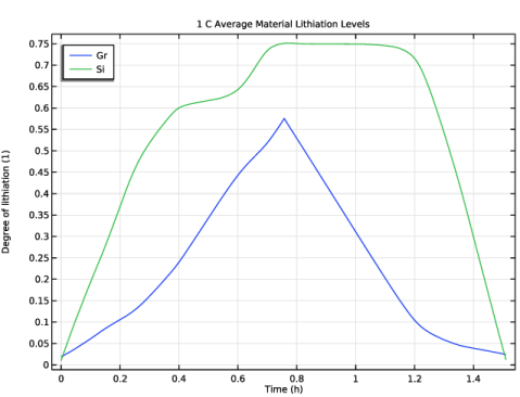
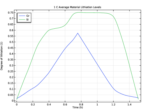
In the Settings window for 1D Plot Group, type 1 C Average Material Lithiation Levels in the Label text field.
3
Locate the Data section. From the Parameter selection (C_rate) list, choose Last.
4
In the 1 C Average Material Lithiation Levels toolbar, click  Plot.
Hysteresis Memory Variable vs. Time
1
In the Results toolbar, click  1D Plot Group.
2
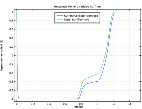
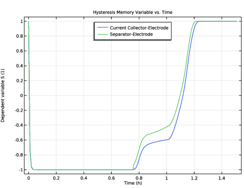
In the Settings window for 1D Plot Group, type Hysteresis Memory Variable vs. Time in the Label text field.
3
Locate the Data section. From the Dataset list, choose Study 1/Parametric Solutions 1 (sol2).
4
From the Parameter selection (C_rate) list, choose From list.
5
In the Parameter values (C_rate) list box, select 1.
6
From the Parameter selection (Si_f) list, choose From list.
7
In the Parameter values (Si_f (%)) list box, select 4.
8
Locate the Title section. From the Title type list, choose Label.
9
Locate the Legend section. From the Position list, choose Upper middle.
Point Graph 1
1
Right-click Hysteresis Memory Variable vs. Time and choose Point Graph.
2
3
In the Settings window for Point Graph, locate the y-Axis Data section.
4
In the Expression text field, type S.
5
Click to expand the Legends section. Select the Show legends checkbox.
6
From the Legends list, choose Manual.
7
8
In the Hysteresis Memory Variable vs. Time toolbar, click  Plot.
Delithiation Energy Densities
1
In the Results toolbar, click  1D Plot Group.
2
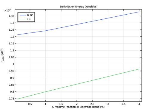
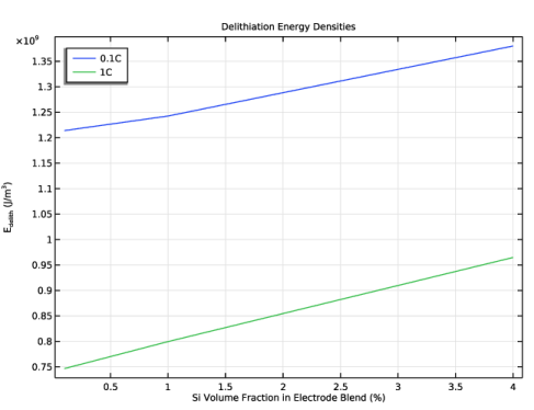
In the Settings window for 1D Plot Group, type Delithiation Energy Densities in the Label text field.
3
Locate the Data section. From the Dataset list, choose None.
4
Locate the Title section. From the Title type list, choose Label.
5
Locate the Plot Settings section.
6
Select the x-axis label checkbox. In the associated text field, type Si Volume Fraction in Electrode Blend (%).
7
Select the y-axis label checkbox. In the associated text field, type E<sub>delith</sub> (J/m<sup>3</sup>).
8
Locate the Legend section. From the Position list, choose Upper left.
Global 1
1
Right-click Delithiation Energy Densities and choose Global.
2
In the Settings window for Global, locate the Data section.
3
From the Dataset list, choose Study 1/Parametric Solutions 1 (sol2).
4
From the Parameter selection (C_rate) list, choose From list.
5
In the Parameter values (C_rate) list box, select 0.1.
6
From the Time selection list, choose Last.
7
Locate the y-Axis Data section. Click  Clear Table.
8
9
Locate the x-Axis Data section. From the Axis source data list, choose Outer solutions.
10
From the Parameter list, choose Expression.
11
Click Replace Expression in the upper-right corner of the x-Axis Data section. From the menu, choose Global definitions > Parameters > Si_f - Fraction of Si in electrode blend - 1.
12
Locate the x-Axis Data section. From the Unit list, choose %.
13
Locate the Legends section. From the Legends list, choose Manual.
14
Global 2
1
Right-click Global 1 and choose Duplicate.
2
In the Settings window for Global, locate the Data section.
3
In the Parameter values (C_rate) list box, select 1.
4
Locate the Legends section. In the table, enter the following settings:
5
In the Delithiation Energy Densities toolbar, click  Plot.
Lithiation/Delithiation Energy Efficiencies
1
In the Model Builder window, right-click Delithiation Energy Densities and choose Duplicate.
2
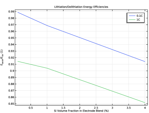
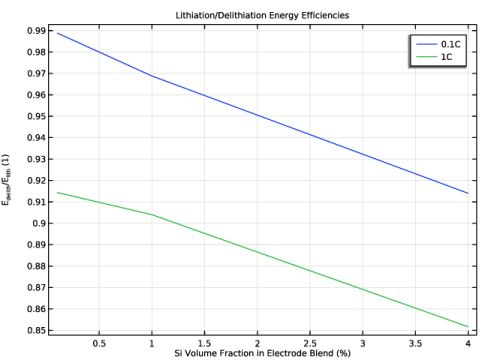
In the Settings window for 1D Plot Group, type Lithiation/Delithiation Energy Efficiencies in the Label text field.
3
Locate the Plot Settings section.
4
Select the y-axis label checkbox. In the associated text field, type E<sub>delith</sub>/E<sub>lith</sub> (1).
5
Locate the Legend section. From the Position list, choose Upper right.
Global 1
1
In the Model Builder window, expand the Lithiation/Delithiation Energy Efficiencies node, then click Global 1.
2
In the Settings window for Global, locate the y-Axis Data section.
3
Global 2
1
In the Model Builder window, click Global 2.
2
In the Settings window for Global, locate the y-Axis Data section.
3
4
In the Lithiation/Delithiation Energy Efficiencies toolbar, click  Plot.
Finally, create a combined plot of the equilibrium potentials of the different materials vs. degree of lithiation.
Definitions (comp1)
Interpolation - Eeq Si Upper (Eeq_Si_upper, Eeq_Si_upper_inv)
1
In the Model Builder window, under Component 1 (comp1) > Definitions click Interpolation - Eeq Si Upper (Eeq_Si_upper, Eeq_Si_upper_inv).
2
In the Settings window for Interpolation, click  Create Plot.
Results
Equilibrium Potentials vs. Lithiation
1
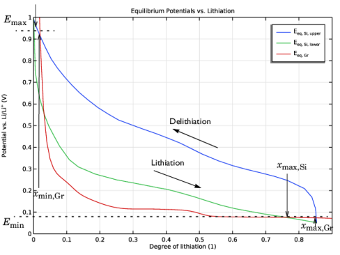
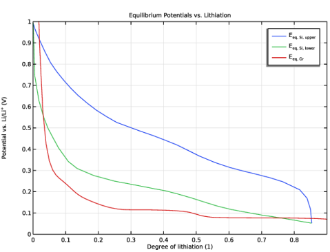
In the Settings window for 1D Plot Group, type Equilibrium Potentials vs. Lithiation in the Label text field.
2
Locate the Data section. From the Dataset list, choose None.
3
Locate the Title section. From the Title type list, choose Label.
4
Locate the Plot Settings section.
5
Select the x-axis label checkbox. In the associated text field, type Degree of lithiation (1).
6
Select the y-axis label checkbox. In the associated text field, type Potential vs. Li/Li<sup>+</sup> (V).
7
Locate the Axis section. Select the Manual axis limits checkbox.
8
In the x minimum text field, type 0.
9
In the x maximum text field, type 0.9.
10
In the y minimum text field, type 0.
11
In the y maximum text field, type 1.
Function 1
1
In the Model Builder window, expand the Equilibrium Potentials vs. Lithiation node, then click Function 1.
2
In the Settings window for Function, locate the Data section.
3
From the Dataset list, choose Grid 1D 1.
4
Locate the y-Axis Data section. Clear the Description checkbox.
5
Locate the Output section. From the Display list, choose Line.
6
From the Extrapolation list, choose None.
7
Click to expand the Legends section. Select the Show legends checkbox.
8
From the Legends list, choose Manual.
9
Definitions (comp1)
Interpolation - Eeq Si Lower (Eeq_Si_lower, Eeq_Si_lower_inv)
1
In the Model Builder window, under Component 1 (comp1) > Definitions click Interpolation - Eeq Si Lower (Eeq_Si_lower, Eeq_Si_lower_inv).
2
In the Settings window for Interpolation, click  Create Plot.
Results
Function 1
In the Model Builder window, expand the 1D Plot Group 16 node, then click Function 1.
Function 2
1
Drag and drop below Equilibrium Potentials vs. Lithiation > Function 1.
2
In the Settings window for Function, locate the Data section.
3
From the Dataset list, choose Grid 1D 1a.
4
Locate the y-Axis Data section. Clear the Description checkbox.
5
Locate the Output section. From the Display list, choose Line.
6
From the Extrapolation list, choose None.
7
Locate the Legends section. Select the Show legends checkbox.
8
From the Legends list, choose Manual.
9
Materials
Graphite, LixC6 MCMB (Negative, Li-ion Battery) (mat1)
In the Model Builder window, expand the Component 1 (comp1) > Materials > Graphite, LixC6 MCMB (Negative, Li-ion Battery) (mat1) node.
Interpolation 3 (Eeq, Eeq_inv)
1
In the Model Builder window, expand the Component 1 (comp1) > Materials > Graphite, LixC6 MCMB (Negative, Li-ion Battery) (mat1) > Basic (def) node, then click Interpolation 3 (Eeq, Eeq_inv).
2
In the Settings window for Interpolation, click  Create Plot.
Results
Function 1
In the Model Builder window, expand the 1D Plot Group 17 node, then click Function 1.
Function 3
1
Drag and drop below Equilibrium Potentials vs. Lithiation > Function 2.
2
In the Settings window for Function, locate the Data section.
3
From the Dataset list, choose Grid 1D 1b.
4
Locate the y-Axis Data section. Clear the Description checkbox.
5
Locate the Legends section. Select the Show legends checkbox.
6
From the Legends list, choose Manual.
7
8
In the Equilibrium Potentials vs. Lithiation toolbar, click  Plot.