PDF

Lithium-Ion Battery with Multiple Intercalating Electrode Materials
Introduction
Lithium-ion batteries can have multiple intercalating materials in both the positive and negative electrodes. For example, the negative electrode can have a mix of different forms of carbon. Similarly, the positive electrode can have a mix of active materials such as transition metal oxides, layered metal oxides, olivines, and so forth. These materials can have different design properties (such as volume fractions, particle sizes), thermodynamic properties (such as equilibrium potentials, maximum lithium concentrations), transport properties (such as solid diffusivities) and kinetic properties (such as intercalation reaction rate constants).
This model example demonstrates the Additional Porous Electrode Material feature in the Lithium-Ion Battery interface. The model describes a lithium-ion battery with two different intercalating materials in the positive electrode, whereas the negative electrode consists of one intercalating material only. The battery performance during discharge for different mixing fractions of the two intercalating materials in the positive electrode is studied. The geometry is in one dimension and the model is isothermal.
Model Definition
This example models the battery cross section in 1D, which implies that edge effects in the length and height of the battery are neglected. The example uses the following three domains:
Separator (50 μm thick)
Two active intercalating materials are considered in the positive electrode and the negative electrode consists of a single intercalating material. The model includes the following processes (Ref. 1).
For the porous electrodes, the effective electrolyte properties are calculated using the Bruggeman relation. Transport in the spherical particles is described using the Baker-Verbrugge diffusion model. This diffusion model considers the gradient of the chemical potential of the intercalating lithium as the driving force for diffusion, as opposed to considering the gradient of lithium concentration for dilute solution treatment (Fick’s Law) of lithium transport in the active material particles. The diffusion equation is expressed in spherical coordinates for the material balance of lithium in the particles. Butler–Volmer electrode kinetics describes the local charge transfer current density in the electrodes. The Butler–Volmer expressions are introduced as source or sink terms in the charge balances and material balances.
Material Properties
The electrolyte consists of 1 M LiPF6 salt in 1:1 EC:DEC (by weight) solvent. The two active materials in the positive electrode are NCA (LiyNi0.80Co0.15Al0.15O2) and LMO (LiyMn2O4 spinel). For the negative electrode, MCMB graphite (LixC6) is used in the model. The material properties of the electrolyte and active materials are taken from the Battery material library.
The equilibrium potentials of the positive electrode materials are shown in Figure 1
Figure 1: The equilibrium potentials of NCA (top) and LMO (bottom).
The x-axis data in Figure 1 depicts the lithiation level of the active material, which is calculated by dividing the concentration of lithium with the maximum concentration of lithium in the material (the host capacity).
Electrode Balancing
The thickness of the negative electrode is set to 50 μm, whereas the positive electrode thickness is set to vary with the relative volume fractions of LMO and NMC. The electrode balancing is based on the following criteria:
Based on the host capacities (cs,max) and volume fractions (εs) of the electrode materials, the thickness of the positive electrode may now be computed as
Results and Discussion
Figure 2 shows the voltage profile for a 1:2 volume ratio of the two positive electrode materials at a constant current discharge of 1C.
Figure 2: Discharge voltage profile at 1C.
Figure 3 shows the lithium concentration at the surface of the active material particles in the positive electrode (at the positive electrode current collector end) during 1C discharge. The variation of the surface concentration with time is different in the two active materials. This is because of the different electrochemical properties of the two active materials.
Figure 3: Surface concentration in the active material particles in the positive electrode during 1C discharge.
Figure 4 shows the lithium concentration inside a particle at a particular position in the negative graphite electrode (at the center of the negative electrode) during 1C discharge. The concentration profiles show characteristic ridges, thereby capturing the staging phenomenon seen in multiphase electrodes like graphite. The Baker–Verbrugge diffusion model accounts for the interactions of the lithium-ions within the solid phase through an activity correction term, and hence provides a realistic representation of the intercalation process.
Figure 4: Concentration profiles inside a particle at a particular position in the negative electrode, at various times during 1C discharge.
The voltage profiles during 1C discharge for different volume mix fractions of the active materials in the positive electrode are shown in Figure 5. The shape of the discharge profile has a pronounced dependence on the mix fraction of the active materials in the electrode.
Figure 5: Voltage profiles during 1C discharge for different volume mix fractions of the active materials in the positive electrode.
Reference
1. P. Albertus, J. Christensen, and J. Newman, “Experiments on and Modeling of Multiple Active Materials in Positive Electrodes for Lithium-Ion Batteries,” J. Electrochem. Soc., vol. 156, no. 7, pp. A606–A618, 2009.
Application Library path: Battery_Design_Module/Lithium-Ion_Batteries,_Performance/li_battery_multiple_materials_1d
Modeling Instructions
From the File menu, choose New.
New
In the New window, click  Model Wizard.
Model Wizard
1
In the Model Wizard window, click  1D.
2
In the Select Physics tree, select Electrochemistry > Batteries > Lithium-Ion Battery (liion).
3
Click Add.
4
Click  Study.
5
In the Select Study tree, select Preset Studies for Selected Physics Interfaces > Time Dependent with Initialization.
6
Global Definitions
Parameters 1
1
In the Model Builder window, under Global Definitions click Parameters 1.
2
In the Settings window for Parameters, locate the Parameters section.
3
Click  Load from File.
4
Geometry 1
The geometry contains three domains. Create the geometry by specifying the coordinates of the boundaries.
Interval 1 (i1)
1
In the Model Builder window, under Component 1 (comp1) right-click Geometry 1 and choose Interval.
2
In the Settings window for Interval, locate the Interval section.
3
From the Specify list, choose Interval lengths.
4
5
Click  Build Selected.
Materials
All materials are available in the Material Library. Note: In the Materials node, cEeqref denotes the maximum lithium concentration in the active material.
Add Material
1
In the Materials toolbar, click  Add Material to open the Add Material window.
2
Go to the Add Material window.
3
In the tree, select Battery > Electrolytes > LiPF6 in 1:1 EC:DEC (Liquid, Li-ion Battery).
4
Click the Add to Component button in the window toolbar.
5
In the tree, select Battery > Electrodes > Graphite, LixC6 MCMB (Negative, Li-ion Battery).
6
Click the Add to Component button in the window toolbar.
7
In the tree, select Battery > Electrodes > NCA, LiNi0.8Co0.15Al0.05O2 (Positive, Li-ion Battery).
8
Click the Add to Component button in the window toolbar.
9
In the tree, select Battery > Electrodes > LMO, LiMn2O4 Spinel (Positive, Li-ion Battery).
10
Click the Add to Component button in the window toolbar.
11
In the Materials toolbar, click  Add Material to close the Add Material window.
Materials
NCA, LiNi0.8Co0.15Al0.05O2 (Positive, Li-ion Battery) (mat3)
In the Model Builder window, expand the NCA, LiNi0.8Co0.15Al0.05O2 (Positive, Li-ion Battery) (mat3) node.
Interpolation 1 (Eeq, Eeq_inv)
1
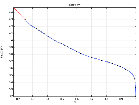
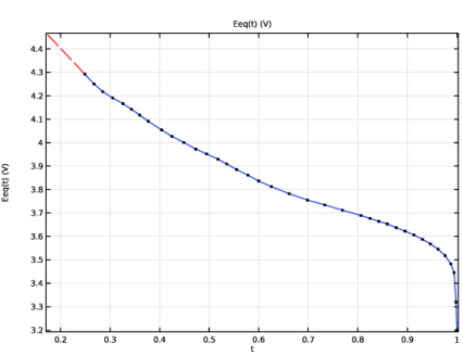
In the Model Builder window, expand the Component 1 (comp1) > Materials > NCA, LiNi0.8Co0.15Al0.05O2 (Positive, Li-ion Battery) (mat3) > Basic (def) node, then click Interpolation 1 (Eeq, Eeq_inv).
2
In the Settings window for Interpolation, click to expand the Plot Parameters section.
3
Clear the Include right extrapolation checkbox.
4
LMO, LiMn2O4 Spinel (Positive, Li-ion Battery) (mat4)
In the Model Builder window, expand the LMO, LiMn2O4 Spinel (Positive, Li-ion Battery) (mat4) node.
Interpolation 1 (Eeq, Eeq_inv)
1
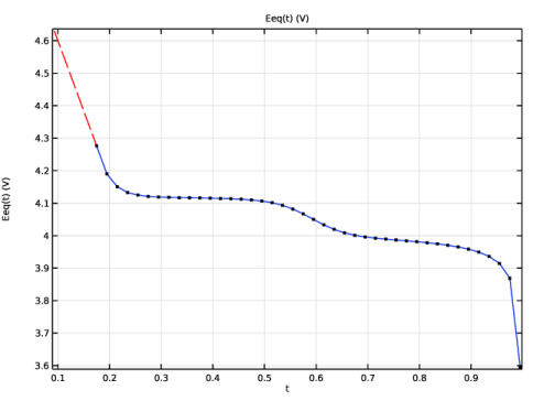
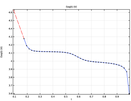
In the Model Builder window, expand the Component 1 (comp1) > Materials > LMO, LiMn2O4 Spinel (Positive, Li-ion Battery) (mat4) > Basic (def) node, then click Interpolation 1 (Eeq, Eeq_inv).
2
In the Settings window for Interpolation, click to expand the Plot Parameters section.
3
Clear the Include right extrapolation checkbox.
4
Lithium-Ion Battery (liion)
Set up the physics in the insertion electrodes. In this model, the Baker-Verbrugge diffusion model is used in the Particle Intercalation nodes. Note that the Baker-Verbrugge diffusivities are typically different from the Fickian diffusivity values. In this model, the intercalation diffusivities are simply set to the values available in the Material Library.
Separator 1
1
In the Model Builder window, under Component 1 (comp1) > Lithium-Ion Battery (liion) click Separator 1.
2
In the Settings window for Separator, locate the Porous Matrix Properties section.
3
In the εl text field, type epsl_sep.
4
Locate the Effective Transport Parameter Correction section. From the Electrolyte conductivity list, choose User defined. In the fl text field, type epsl_sep^brugl_sep.
5
From the Diffusion list, choose User defined. In the fDl text field, type epsl_sep^brugl_sep.
Porous Electrode 1
1
In the Physics toolbar, click  Domains and choose Porous Electrode.
2
3
In the Settings window for Porous Electrode, locate the Electrode Properties section.
4
In the σs text field, type sigmas_neg.
5
Locate the Porous Matrix Properties section. In the εs text field, type epss_neg.
6
In the εl text field, type epsl_neg.
Particle Intercalation 1
1
In the Model Builder window, click Particle Intercalation 1.
2
In the Settings window for Particle Intercalation, locate the Material section.
3
From the Particle material list, choose Graphite, LixC6 MCMB (Negative, Li-ion Battery) (mat2).
4
Locate the Particle Transport Properties section. From the Species concentration transport model list, choose Baker–Verbrugge.
5
In the rp text field, type rp_neg.
The concentration profiles inside a graphite electrode particle will be analyzed during postprocessing. Hence, it is useful to have a finer resolution along the particle dimension, by setting a linear distribution with 20 elements.
6
Click to expand the Particle Discretization section. From the Distribution list, choose Linear.
7
In the Nel text field, type 20.
Porous Electrode Reaction 1
1
In the Model Builder window, click Porous Electrode Reaction 1.
2
In the Settings window for Porous Electrode Reaction, locate the Material section.
3
From the Material list, choose Graphite, LixC6 MCMB (Negative, Li-ion Battery) (mat2).
4
Locate the Electrode Kinetics section. In the i0,ref(T) text field, type i0ref_neg.
Porous Electrode 2
1
In the Physics toolbar, click  Domains and choose Porous Electrode.
2
3
In the Settings window for Porous Electrode, locate the Electrode Properties section.
4
In the σs text field, type sigmas_pos.
5
Locate the Porous Matrix Properties section. In the εs text field, type epss_pos_NCA.
6
In the εl text field, type epsl_pos.
7
Locate the Effective Transport Parameter Correction section. From the Electrolyte conductivity list, choose User defined. In the fl text field, type epsl_pos^brugl_pos.
8
From the Diffusion list, choose User defined. In the fDl text field, type epsl_pos^brugl_pos.
Particle Intercalation 1
1
In the Model Builder window, click Particle Intercalation 1.
2
In the Settings window for Particle Intercalation, locate the Material section.
3
From the Particle material list, choose NCA, LiNi0.8Co0.15Al0.05O2 (Positive, Li-ion Battery) (mat3).
4
Locate the Particle Transport Properties section. From the Species concentration transport model list, choose Baker–Verbrugge.
5
In the rp text field, type rp_pos_NCA.
Porous Electrode Reaction 1
1
In the Model Builder window, click Porous Electrode Reaction 1.
2
In the Settings window for Porous Electrode Reaction, locate the Material section.
3
From the Material list, choose NCA, LiNi0.8Co0.15Al0.05O2 (Positive, Li-ion Battery) (mat3).
4
Locate the Electrode Kinetics section. In the i0,ref(T) text field, type i0ref_pos_NCA.
Additional Porous Electrode Material 1
1
In the Physics toolbar, click  Domains and choose Additional Porous Electrode Material.
2
3
In the Settings window for Additional Porous Electrode Material, locate the Volume Fraction section.
4
In the εs text field, type epss_pos_LMO.
Particle Intercalation 1
1
In the Model Builder window, click Particle Intercalation 1.
2
In the Settings window for Particle Intercalation, locate the Material section.
3
From the Particle material list, choose LMO, LiMn2O4 Spinel (Positive, Li-ion Battery) (mat4).
4
Locate the Particle Transport Properties section. From the Species concentration transport model list, choose Baker–Verbrugge.
5
In the rp text field, type rp_pos_LMO.
Porous Electrode Reaction 1
1
In the Model Builder window, click Porous Electrode Reaction 1.
2
In the Settings window for Porous Electrode Reaction, locate the Material section.
3
From the Material list, choose LMO, LiMn2O4 Spinel (Positive, Li-ion Battery) (mat4).
4
Locate the Electrode Kinetics section. In the i0,ref(T) text field, type i0ref_pos_LMO.
5
In the Model Builder window, click Lithium-Ion Battery (liion).
6
In the Settings window for Lithium-Ion Battery, locate the Cell Settings section.
7
Select the Define cell state of charge (SOC) and initial charge inventory checkbox.
SOC and Initial Charge Distribution 1
1
In the Model Builder window, expand the Lithium-Ion Battery (liion) node, then click SOC and Initial Charge Distribution 1.
2
In the Settings window for SOC and Initial Charge Distribution, locate the State-of-Charge Definition section.
3
From the list, choose User defined. In the Ecell0%SOC text field, type E_0_SOC.
4
In the Ecell100%SOC text field, type E_100_SOC.
5
Locate the Initial Cell Charge Distribution section. In the SOC0 text field, type SOC_cell0.
Negative Electrode Domain Selection 1
1
In the Model Builder window, click Negative Electrode Domain Selection 1.
2
Positive Electrode Domain Selection 1
1
In the Model Builder window, click Positive Electrode Domain Selection 1.
2
Electric Ground 1
1
In the Physics toolbar, click  Boundaries and choose Electric Ground.
2
Load Cycle 1
1
In the Physics toolbar, click  Boundaries and choose Load Cycle.
2
3
In the Settings window for Load Cycle, locate the Load Type section.
4
5
Locate the Cycling Stop Condition section. From the list, choose Minimum voltage.
6
In the Emin text field, type 3[V].
C Rate 1
1
In the Physics toolbar, click  Attributes and choose C Rate.
2
In the Settings window for C Rate, locate the C-Rate Multiple section.
3
In the Cset text field, type -1.
Global Definitions
Default Model Inputs
Set up the temperature value used in the entire model.
1
In the Model Builder window, under Global Definitions click Default Model Inputs.
2
In the Settings window for Default Model Inputs, locate the Browse Model Inputs section.
3
In the tree, select General > Temperature (K) - minput.T.
4
Find the Expression for remaining selection subsection. In the Temperature text field, type T.
Mesh 1
1
In the Model Builder window, under Component 1 (comp1) click Mesh 1.
2
In the Settings window for Mesh, locate the Physics-Controlled Mesh section.
3
From the Element size list, choose Fine.
4
Click  Build All.
Study 1
Step 2: Time Dependent
1
In the Model Builder window, under Study 1 click Step 2: Time Dependent.
2
In the Settings window for Time Dependent, locate the Study Settings section.
3
In the Output times text field, type 0 3600.
Store the actual steps taken by the solver to make sure to capture any sudden steep voltage changes.
Solution 1 (sol1)
1
In the Study toolbar, click  Show Default Solver.
2
In the Model Builder window, expand the Solution 1 (sol1) node, then click Time-Dependent Solver 1.
3
In the Settings window for Time-Dependent Solver, locate the General section.
4
From the Times to store list, choose Steps taken by solver.
5
In the Model Builder window, click Study 1.
6
In the Settings window for Study, locate the Study Settings section.
7
Clear the Generate default plots checkbox.
8
In the Study toolbar, click  Compute.
Results
Reproduce the plots in the model documentation for 1C discharge, starting with the voltage profile (Figure 2).
Constant current 1C Discharge
1
In the Results toolbar, click  1D Plot Group.
2
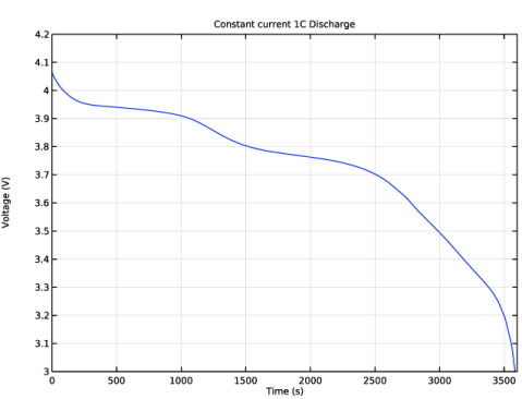
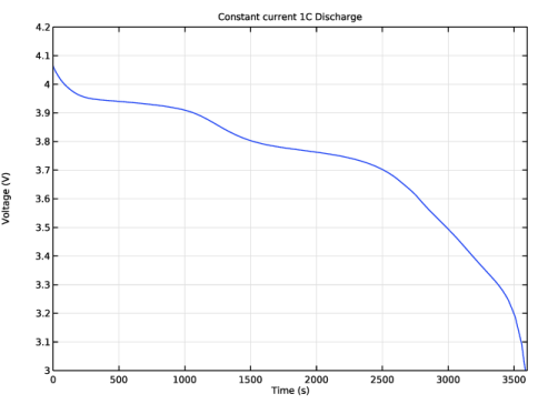
In the Settings window for 1D Plot Group, type Constant current 1C Discharge in the Label text field.
Point Graph 1
1
Right-click Constant current 1C Discharge and choose Point Graph.
2
3
In the Settings window for Point Graph, click Replace Expression in the upper-right corner of the y-Axis Data section. From the menu, choose Component 1 (comp1) > Lithium-Ion Battery > phis - Electric potential - V.
Constant current 1C Discharge
1
In the Model Builder window, click Constant current 1C Discharge.
2
In the Settings window for 1D Plot Group, click to expand the Title section.
3
From the Title type list, choose Label.
4
Locate the Plot Settings section.
5
Select the y-axis label checkbox. In the associated text field, type Voltage (V).
6
Locate the Axis section. Select the Manual axis limits checkbox.
7
In the x minimum text field, type 0.
8
In the x maximum text field, type 3600.
9
In the y minimum text field, type 3.0.
10
In the y maximum text field, type 4.2.
11
In the Constant current 1C Discharge toolbar, click  Plot.
Surface concentration Positive
The following steps are for plotting the surface concentration in each active material in the positive electrode during 1C discharge (Figure 3).
1
In the Results toolbar, click  1D Plot Group.
2
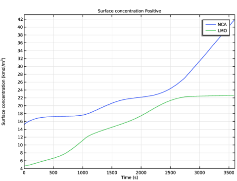
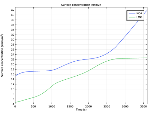
In the Settings window for 1D Plot Group, type Surface concentration Positive in the Label text field.
Point Graph 1
1
Right-click Surface concentration Positive and choose Point Graph.
2
3
In the Settings window for Point Graph, click Replace Expression in the upper-right corner of the y-Axis Data section. From the menu, choose Component 1 (comp1) > Lithium-Ion Battery > Particle intercalation > liion.cs_surface - Insertion particle concentration, surface - mol/m³.
4
Locate the y-Axis Data section. From the Unit list, choose M.
5
Click to expand the Legends section. Select the Show legends checkbox.
6
From the Legends list, choose Manual.
7
Point Graph 2
1
Right-click Point Graph 1 and choose Duplicate.
2
In the Settings window for Point Graph, click Replace Expression in the upper-right corner of the y-Axis Data section. From the menu, choose Component 1 (comp1) > Lithium-Ion Battery > Particle intercalation > liion.cs_surface_addm1 - Insertion particle surface concentration, Additional Porous Electrode Material 1 - mol/m³.
3
Locate the Legends section. In the table, enter the following settings:
Surface concentration Positive
1
In the Model Builder window, click Surface concentration Positive.
2
In the Settings window for 1D Plot Group, locate the Title section.
3
From the Title type list, choose Label.
4
Locate the Plot Settings section.
5
Select the y-axis label checkbox. In the associated text field, type Surface concentration (kmol/m<sup>3</sup>).
6
Locate the Axis section. Select the Manual axis limits checkbox.
7
In the x minimum text field, type 0.
8
In the x maximum text field, type 3600.
9
In the y minimum text field, type 4.
10
In the Surface concentration Positive toolbar, click  Plot.
Study 1/Solution 1 (sol1)
The following steps are for plotting the concentration profiles inside a particle at a particular position in the negative electrode, at various times during 1C discharge (Figure 4). To do this, create a solution dataset that refers to the extra dimension that is set up by the Porous Electrode node corresponding to the negative electrode.
Study 1/Solution 1: xdim Negative
1
In the Model Builder window, expand the Results > Datasets node.
2
Right-click Results > Datasets > Study 1/Solution 1 (sol1) and choose Duplicate.
3
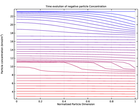
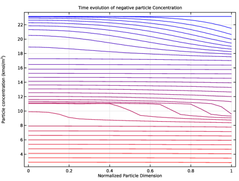
In the Settings window for Solution, type Study 1/Solution 1: xdim Negative in the Label text field.
4
Locate the Solution section. From the Component list, choose Extra Dimension from Particle Intercalation 1 (liion_pce1_pin1_xdim).
Time evolution of negative particle Concentration
1
In the Results toolbar, click  1D Plot Group.
2
In the Settings window for 1D Plot Group, type Time evolution of negative particle Concentration in the Label text field.
3
Locate the Data section. From the Dataset list, choose Study 1/Solution 1: xdim Negative (sol1).
4
From the Time selection list, choose Interpolated.
5
In the Times (s) text field, type range(0,100,3300).
Line Graph 1
1
Right-click Time evolution of negative particle Concentration and choose Line Graph.
2
The atxd1() operator evaluates the concentration at a specified position inside the negative electrode over the length of the particle dimension.
3
In the Settings window for Line Graph, locate the y-Axis Data section.
4
In the Expression text field, type atxd1(25e-6,liion.cs_pce1).
5
From the Unit list, choose M.
6
Click to expand the Coloring and Style section. From the Color list, choose Gradient.
7
From the Top color list, choose Red.
8
From the Bottom color list, choose Blue.
Time evolution of negative particle Concentration
1
In the Model Builder window, click Time evolution of negative particle Concentration.
2
In the Settings window for 1D Plot Group, locate the Title section.
3
From the Title type list, choose Label.
4
Locate the Plot Settings section.
5
Select the x-axis label checkbox. In the associated text field, type Normalized Particle Dimension.
6
Select the y-axis label checkbox. In the associated text field, type Particle concentration (kmol/m<sup>3</sup>).
7
In the Time evolution of negative particle Concentration toolbar, click  Plot.
Root
Now set up a parametric study for different mix fractions of active materials in the positive electrode.
Add Study
1
In the Home toolbar, click  Add Study to open the Add Study window.
2
Go to the Add Study window.
3
Find the Studies subsection. In the Select Study tree, select Preset Studies for Selected Physics Interfaces > Time Dependent with Initialization.
4
Click the Add Study button in the window toolbar.
5
In the Home toolbar, click  Add Study to close the Add Study window.
Study 2
Step 2: Time Dependent
1
In the Model Builder window, under Study 2 click Step 2: Time Dependent.
2
In the Settings window for Time Dependent, locate the Study Settings section.
3
In the Output times text field, type 0 3600.
Parametric Sweep
1
In the Study toolbar, click  Parametric Sweep.
2
In the Settings window for Parametric Sweep, locate the Study Settings section.
3
4
Solution 3 (sol3)
1
In the Study toolbar, click  Show Default Solver.
2
In the Model Builder window, expand the Solution 3 (sol3) node, then click Time-Dependent Solver 1.
3
In the Settings window for Time-Dependent Solver, locate the General section.
4
From the Times to store list, choose Steps taken by solver.
Store only every 3rd time step. This reduces the size of the stored solution and the size of model file.
5
In the Store every Nth step text field, type 3.
6
In the Model Builder window, click Study 2.
7
In the Settings window for Study, locate the Study Settings section.
8
Clear the Generate default plots checkbox.
9
In the Study toolbar, click  Compute.
Results
You can plot the voltage profiles from the parametric study (Figure 5) by performing the following steps:
Voltage profiles for different mix fractions of NCA and LMO
1
In the Results toolbar, click  1D Plot Group.
2
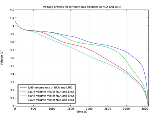
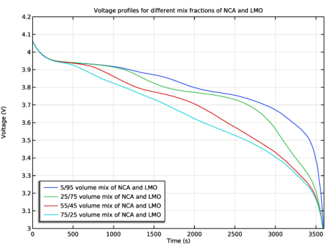
In the Settings window for 1D Plot Group, type Voltage profiles for different mix fractions of NCA and LMO in the Label text field.
Point Graph 1
1
Right-click Voltage profiles for different mix fractions of NCA and LMO and choose Point Graph.
2
In the Settings window for Point Graph, locate the Data section.
3
From the Dataset list, choose Study 2/Parametric Solutions 1 (sol5).
4
5
Click Replace Expression in the upper-right corner of the y-Axis Data section. From the menu, choose phis - Electric potential - V.
6
Locate the Legends section. Select the Show legends checkbox.
7
From the Legends list, choose Evaluated.
8
In the Legend text field, type eval(fr_pos_NCA*100)/eval((1-fr_pos_NCA)*100) volume mix of NCA and LMO.
Voltage profiles for different mix fractions of NCA and LMO
1
In the Model Builder window, click Voltage profiles for different mix fractions of NCA and LMO.
2
In the Settings window for 1D Plot Group, locate the Plot Settings section.
3
Select the y-axis label checkbox. In the associated text field, type Voltage (V).
4
Locate the Title section. From the Title type list, choose Label.
5
Locate the Axis section. Select the Manual axis limits checkbox.
6
In the x minimum text field, type 0.
7
In the x maximum text field, type 3600.
8
In the y minimum text field, type 3.0.
9
In the y maximum text field, type 4.2.
10
Locate the Legend section. From the Position list, choose Lower left.
11
In the Voltage profiles for different mix fractions of NCA and LMO toolbar, click  Plot.