|
|
|

|
1
|
|
2
|
|
3
|
Click Add.
|
|
4
|
|
5
|
In the Select Physics tree, select Chemical Species Transport > Transport of Diluted Species in Porous Media (tds).
|
|
6
|
Click Add.
|
|
7
|
In the Concentrations (mol/m³) table, enter the following settings:
|
|
8
|
In the Select Physics tree, select Mathematics > ODE and DAE Interfaces > Domain ODEs and DAEs (dode).
|
|
9
|
Click Add.
|
|
10
|
In the Dependent variables (1) table, enter the following settings:
|
|
11
|
Click
|
|
12
|
|
13
|
|
14
|
Click OK.
|
|
15
|
|
16
|
|
17
|
|
18
|
Click OK.
|
|
19
|
|
20
|
|
21
|
Click
|
|
1
|
|
2
|
|
3
|
Click
|
|
4
|
Browse to the model’s Application Libraries folder and double-click the file li_air_battery_1d_parameters.txt.
|
|
1
|
|
2
|
|
3
|
|
5
|
|
1
|
|
2
|
|
3
|
|
5
|
|
6
|
Browse to the model’s Application Libraries folder and double-click the file li_air_battery_1d_variables.txt.
|
|
1
|
|
2
|
|
3
|
|
1
|
In the Model Builder window, under Component 1 (comp1) > Lithium-Ion Battery (liion) click Separator 1.
|
|
2
|
|
3
|
|
4
|
|
5
|
|
6
|
|
7
|
|
1
|
|
3
|
|
4
|
|
5
|
|
6
|
|
7
|
|
8
|
|
9
|
|
10
|
|
11
|
|
12
|
|
14
|
Clear the Add volume change to electrode volume fraction checkbox.
|
|
15
|
Click to expand the Film Resistance section. From the Film resistance list, choose Surface resistance.
|
|
16
|
|
1
|
|
2
|
|
3
|
|
4
|
Locate the Electrode Kinetics section. From the Kinetics expression type list, choose Concentration dependent kinetics.
|
|
5
|
|
6
|
|
7
|
|
8
|
|
9
|
|
10
|
Locate the Active Specific Surface Area section. From the Active specific surface area list, choose User defined. In the av text field, type apos.
|
|
11
|
|
12
|
|
13
|
In the Stoichiometric coefficients for dissolving–depositing species: table, enter the following settings:
|
|
14
|
|
1
|
|
1
|
|
2
|
|
3
|
From the Eeq list, choose User defined. Locate the Electrode Kinetics section. In the i0,ref(T) text field, type i0refLi.
|
|
4
|
|
1
|
|
3
|
|
4
|
|
1
|
|
2
|
|
3
|
|
4
|
|
1
|
|
3
|
|
4
|
|
1
|
In the Model Builder window, under Component 1 (comp1) click Transport of Diluted Species in Porous Media (tds).
|
|
3
|
In the Settings window for Transport of Diluted Species in Porous Media, locate the Transport Mechanisms section.
|
|
4
|
Clear the Convection checkbox.
|
|
5
|
|
1
|
|
2
|
|
3
|
|
4
|
|
1
|
|
2
|
|
3
|
|
1
|
|
3
|
|
4
|
Select the Species cO2 checkbox.
|
|
5
|
|
1
|
|
2
|
|
3
|
|
1
|
|
1
|
In the Model Builder window, expand the Porous Electrode Coupling 1 node, then click Reaction Coefficients 1.
|
|
2
|
|
3
|
|
4
|
|
5
|
|
1
|
|
2
|
In the Settings window for Domain ODEs and DAEs, type Domain ODEs and DAEs: Concentration of Li2O2 in the Label text field.
|
|
4
|
|
1
|
In the Model Builder window, under Component 1 (comp1) > Domain ODEs and DAEs: Concentration of Li2O2 (dode) click Distributed ODE 1.
|
|
2
|
|
3
|
|
1
|
|
2
|
|
3
|
|
4
|
|
1
|
|
2
|
|
3
|
|
4
|
Click
|
|
1
|
|
2
|
|
3
|
Click
|
|
1
|
|
2
|
|
3
|
|
4
|
|
5
|
|
1
|
|
2
|
|
3
|
|
4
|
|
5
|
|
6
|
Right-click Study 1 > Solver Configurations > Solution 1 (sol1) > Time-Dependent Solver 1 and choose Stop Condition.
|
|
7
|
|
8
|
Click
|
|
10
|
|
11
|
|
12
|
|
13
|
Clear the Generate default plots checkbox.
|
|
14
|
|
1
|
|
2
|
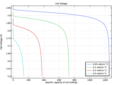
In the Settings window for 1D Plot Group, type Cell Voltages for different iapp in the Label text field.
|
|
3
|
|
1
|
|
3
|
In the Settings window for Point Graph, click Replace Expression in the upper-right corner of the y-Axis Data section. From the menu, choose Component 1 (comp1) > Lithium-Ion Battery > phis - Electric potential - V.
|
|
4
|
|
5
|
Click Replace Expression in the upper-right corner of the x-Axis Data section. From the menu, choose Component 1 (comp1) > Definitions > Variables > capacity - Specific capacity of cell - C/kg.
|
|
6
|
|
7
|
|
8
|
|
1
|
|
2
|
|
3
|
Select the x-axis label checkbox. In the associated text field, type Specific capacity of cell (mAh/g).
|
|
4
|
|
5
|
|
6
|
|
7
|
|
8
|
|
1
|
|
2
|
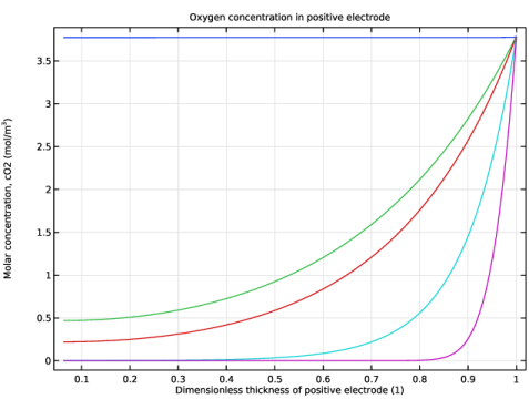
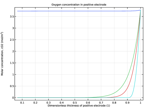
In the Settings window for 1D Plot Group, type Oxygen conc in positive electrode, iapp = 0.1mA/cm2 in the Label text field.
|
|
3
|
|
4
|
|
5
|
|
6
|
|
7
|
|
1
|
|
3
|
In the Settings window for Line Graph, click Replace Expression in the upper-right corner of the y-Axis Data section. From the menu, choose Component 1 (comp1) > Transport of Diluted Species in Porous Media > Species cO2 > cO2 - Molar concentration, cO2 - mol/m³.
|
|
4
|
|
5
|
|
6
|
Select the Description checkbox. In the associated text field, type Dimensionless thickness of positive electrode.
|
|
1
|
|
2
|
|
3
|
|
4
|
|
5
|
|
1
|
|
2
|
In the Settings window for 1D Plot Group, type Oxygen conc in positive electrode, iapp = 0.5mA/cm2 in the Label text field.
|
|
3
|
|
4
|
|
5
|
|
6
|
|
1
|
|
2
|
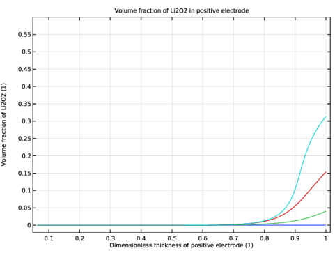
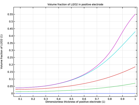
In the Settings window for 1D Plot Group, type Volume fraction of Li2O2 in positive electrode, iapp = 0.1mA/cm2 in the Label text field.
|
|
3
|
|
4
|
|
5
|
|
6
|
|
7
|
|
1
|
|
3
|
In the Settings window for Line Graph, click Replace Expression in the upper-right corner of the y-Axis Data section. From the menu, choose Component 1 (comp1) > Definitions > Variables > epsilonLi2O2 - Volume fraction of Li2O2 - 1.
|
|
4
|
|
5
|
|
6
|
Select the Description checkbox. In the associated text field, type Dimensionless thickness of positive electrode.
|
|
1
|
In the Model Builder window, click Volume fraction of Li2O2 in positive electrode, iapp = 0.1mA/cm2.
|
|
2
|
|
3
|
|
4
|
|
5
|
|
6
|
|
7
|
|
1
|
|
2
|
In the Settings window for 1D Plot Group, type Volume fraction of Li2O2 in positive electrode, iapp = 0.5mA/cm2 in the Label text field.
|
|
3
|
|
4
|
|
5
|
|
1
|
|
2
|
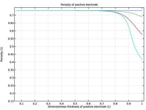
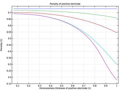
In the Settings window for 1D Plot Group, type Porosity of positive electrode, iapp = 0.1mA/cm2 in the Label text field.
|
|
3
|
|
4
|
|
5
|
|
6
|
|
7
|
|
1
|
|
3
|
|
4
|
|
5
|
|
6
|
|
7
|
|
8
|
Select the Description checkbox. In the associated text field, type Dimensionless thickness of positive electrode.
|
|
1
|
|
2
|
|
3
|
|
4
|
|
5
|
|
6
|
|
7
|
|
8
|
|
1
|
|
2
|
In the Settings window for 1D Plot Group, type Porosity of positive electrode, iapp = 0.5mA/cm2 in the Label text field.
|
|
3
|
|
4
|
|
5
|