|
|
|

|
1
|
|
2
|
|
3
|
Click Add.
|
|
4
|
|
5
|
Click Add.
|
|
6
|
Click
|
|
7
|
In the Select Study tree, select Preset Studies for Selected Physics Interfaces > Lithium-Ion Battery > Time Dependent with Initialization.
|
|
8
|
Click
|
|
1
|
|
2
|
Browse to the model’s Application Libraries folder and double-click the file heterogeneous_lib_geom_sequence.mph.
|
|
3
|
|
4
|
Click OK.
|
|
5
|
|
6
|
|
7
|
|
8
|
|
9
|
|
10
|
|
1
|
|
2
|
|
1
|
|
2
|
|
3
|
|
4
|
Browse to the model’s Application Libraries folder and double-click the file heterogeneous_lib_physics_parameters.txt.
|
|
1
|
|
2
|
Go to the Add Material window.
|
|
3
|
|
4
|
Right-click and choose Add to Component 1 (comp1).
|
|
5
|
|
6
|
Right-click and choose Add to Component 1 (comp1).
|
|
7
|
In the tree, select Battery > Electrodes > NMC 111, LiNi0.33Mn0.33Co0.33O2 (Positive, Li-ion Battery).
|
|
8
|
Right-click and choose Add to Component 1 (comp1).
|
|
9
|
|
10
|
Right-click and choose Add to Component 1 (comp1).
|
|
11
|
|
1
|
|
2
|
|
3
|
In the Model Builder window, expand the Graphite, LixC6 MCMB (Negative, Li-ion Battery) (mat1) node.
|
|
1
|
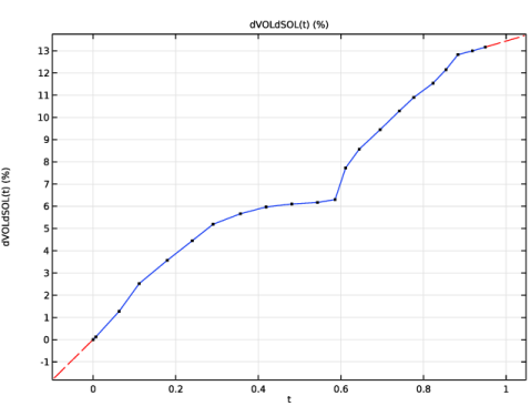
In the Model Builder window, expand the Component 1 (comp1) > Materials > Graphite, LixC6 MCMB (Negative, Li-ion Battery) (mat1) > Intercalation strain (is) node, then click Interpolation 1 (dVOLdSOL).
|
|
2
|
|
1
|
|
2
|
|
3
|
|
1
|
In the Model Builder window, click NMC 111, LiNi0.33Mn0.33Co0.33O2 (Positive, Li-ion Battery) (mat3).
|
|
2
|
|
3
|
|
1
|
|
2
|
|
3
|
|
1
|
In the Model Builder window, under Component 1 (comp1) > Materials right-click Graphite, LixC6 MCMB (Negative, Li-ion Battery) (mat1) and choose Duplicate.
|
|
2
|
|
3
|
|
4
|
|
1
|
In the Model Builder window, under Component 1 (comp1) > Materials right-click Silicon, LixSi (Negative, Li-ion Battery) (mat2) and choose Duplicate.
|
|
2
|
|
3
|
|
4
|
|
1
|
In the Model Builder window, under Component 1 (comp1) > Materials right-click NMC 111, LiNi0.33Mn0.33Co0.33O2 (Positive, Li-ion Battery) (mat3) and choose Duplicate.
|
|
2
|
|
3
|
|
4
|
|
1
|
|
2
|
|
3
|
|
4
|
|
5
|
|
6
|
|
1
|
In the Model Builder window, under Component 1 (comp1) > Lithium-Ion Battery (liion) click Separator 1.
|
|
2
|
|
3
|
|
1
|
|
2
|
|
3
|
|
4
|
|
5
|
|
6
|
|
7
|
Locate the Effective Transport Parameter Correction section. From the Electric conductivity list, choose No correction.
|
|
1
|
|
2
|
|
3
|
|
1
|
|
2
|
|
3
|
|
4
|
Locate the Electrode Kinetics section. From the Kinetics expression type list, choose Lithium insertion.
|
|
5
|
|
1
|
|
2
|
|
3
|
|
1
|
|
2
|
|
3
|
|
4
|
|
5
|
|
1
|
|
2
|
|
3
|
|
1
|
|
2
|
|
3
|
Locate the Diffusion section. From the Material list, choose Graphite, LixC6 MCMB (Negative, Li-ion Battery) (mat1).
|
|
4
|
|
1
|
|
2
|
|
3
|
|
4
|
Locate the Diffusion section. From the Material list, choose Silicon, LixSi (Negative, Li-ion Battery) (mat2).
|
|
5
|
|
1
|
|
2
|
|
3
|
|
4
|
Locate the Diffusion section. From the Material list, choose NMC 111, LiNi0.33Mn0.33Co0.33O2 (Positive, Li-ion Battery) (mat3).
|
|
5
|
|
1
|
|
2
|
|
3
|
|
4
|
Locate the Reaction section. From the iloc list, choose Local current density, Electrode Reaction 1 (liion/bei1/er1).
|
|
5
|
|
6
|
|
1
|
|
2
|
|
3
|
|
4
|
|
1
|
|
2
|
|
3
|
|
4
|
|
1
|
|
2
|
|
3
|
|
1
|
|
2
|
|
3
|
From the list, choose User-controlled mesh.
|
|
4
|
|
1
|
|
2
|
|
3
|
|
4
|
|
5
|
|
1
|
|
2
|
|
3
|
Click the Custom button.
|
|
4
|
Locate the Element Size Parameters section. In the Maximum element size text field, type s_unit_cell/3.
|
|
5
|
|
6
|
|
7
|
|
8
|
|
9
|
|
10
|
|
1
|
|
2
|
In the Settings window for Global Variable Probe, click Replace Expression in the upper-right corner of the Expression section. From the menu, choose Component 1 (comp1) > Lithium-Ion Battery > liion.phis0_ec1 - Electric potential on boundary - V.
|
|
3
|
Locate the Expression section.
|
|
4
|
|
1
|
|
2
|
|
3
|
|
4
|
|
5
|
|
6
|
Clear the Generate default plots checkbox.
|
|
7
|
|
1
|
|
2
|
|
3
|
|
1
|
|
2
|
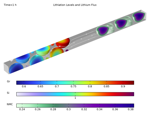
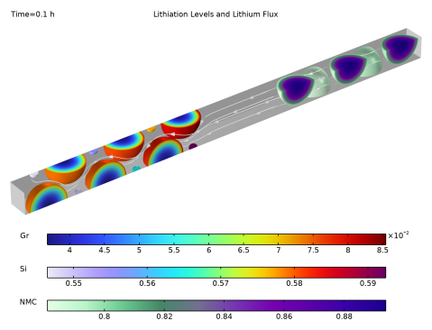
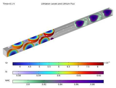
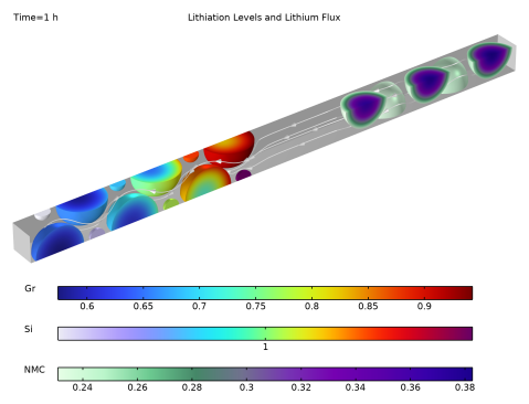
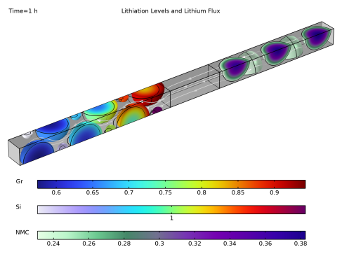
In the Settings window for 3D Plot Group, type Lithiation Levels and Lithium Flux in the Label text field.
|
|
3
|
|
4
|
|
5
|
|
6
|
|
1
|
|
2
|
|
3
|
|
4
|
|
1
|
|
2
|
|
3
|
|
1
|
In the Model Builder window, under Results > Lithiation Levels and Lithium Flux right-click Volume 1 and choose Duplicate.
|
|
2
|
|
3
|
|
4
|
|
5
|
|
1
|
|
2
|
|
3
|
|
1
|
In the Model Builder window, under Results > Lithiation Levels and Lithium Flux right-click Volume 2 and choose Duplicate.
|
|
2
|
|
3
|
|
4
|
|
5
|
|
6
|
|
1
|
|
2
|
|
3
|
|
4
|
|
1
|
|
2
|
In the Settings window for Streamline, click Replace Expression in the upper-right corner of the Expression section. From the menu, choose Component 1 (comp1) > Lithium-Ion Battery > liion.Nposx,...,liion.Nposz - Positive ion flux.
|
|
3
|
|
5
|
Locate the Coloring and Style section. Find the Point style subsection. From the Type list, choose Arrow.
|
|
6
|
|
7
|
|
1
|
|
2
|
|
3
|
|
4
|
|
5
|
|
1
|
|
3
|
|
4
|
|
1
|
|
2
|
|
3
|
|
4
|
|
1
|
|
2
|
|
3
|
|
4
|
|
5
|
|
6
|
|
1
|
|
2
|
Go to the Add Physics window.
|
|
3
|
|
4
|
Click the Add to Component 1 button in the window toolbar.
|
|
5
|
|
1
|
|
2
|
From the list, choose Quasistatic.
|
|
1
|
In the Model Builder window, under Component 1 (comp1) > Solid Mechanics (solid) click Linear Elastic Material 1.
|
|
2
|
|
3
|
|
4
|
|
5
|
|
1
|
|
2
|
|
3
|
|
4
|
|
1
|
|
2
|
|
3
|
|
1
|
|
2
|
|
3
|
|
4
|
Locate the Linear Elastic Material section. From the E list, choose User defined. In the associated text field, type E_sep.
|
|
5
|
|
6
|
|
1
|
|
3
|
|
4
|
|
5
|
|
6
|
|
7
|
|
1
|
|
2
|
|
3
|
|
1
|
|
2
|
|
3
|
|
1
|
In the Model Builder window, under Component 1 (comp1) > Materials click Silicon, LixSi (Negative, Li-ion Battery) (mat2).
|
|
2
|
|
1
|
In the Model Builder window, click NMC 111, LiNi0.33Mn0.33Co0.33O2 (Positive, Li-ion Battery) (mat3).
|
|
2
|
|
1
|
In the Model Builder window, under Component 1 (comp1) right-click Definitions and choose Variables.
|
|
2
|
|
3
|
|
4
|
|
5
|
Locate the Variables section. In the table, enter the following settings:
|
|
1
|
|
2
|
In the Settings window for Variables, type Variables - Porous Conductive Binder in the Label text field.
|
|
3
|
Locate the Geometric Entity Selection section. From the Selection list, choose Porous Conductive Binder.
|
|
4
|
Locate the Variables section. In the table, enter the following settings:
|
|
1
|
In the Model Builder window, under Component 1 (comp1) > Lithium-Ion Battery (liion) click Separator 1.
|
|
2
|
|
3
|
|
1
|
|
2
|
|
3
|
|
4
|
|
1
|
|
2
|
Go to the Add Study window.
|
|
3
|
Find the Studies subsection. In the Select Study tree, select Preset Studies for Selected Physics Interfaces > Lithium-Ion Battery > Time Dependent with Initialization.
|
|
4
|
Right-click and choose Add Study.
|
|
5
|
|
1
|
In the Model Builder window, under Component 1 (comp1) > Definitions right-click Global Variable Probe 1 (var1) and choose Duplicate.
|
|
2
|
In the Settings window for Global Variable Probe, click to expand the Table and Window Settings section.
|
|
3
|
Click
|
|
1
|
|
2
|
|
3
|
|
4
|
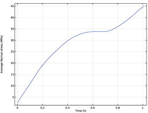
Click Replace Expression in the upper-right corner of the Expression section. From the menu, choose Component 1 (comp1) > Solid Mechanics > Stress > solid.stn - Normal stress - N/m².
|
|
5
|
|
6
|
|
7
|
|
8
|
Click
|
|
1
|
|
2
|
|
1
|
In the Model Builder window, under Study 1 - Excluding Solid Mechanics click Step 2: Time Dependent.
|
|
2
|
|
3
|
In the Solve for column of the table, under Component 1 (comp1), clear the checkbox for Solid Mechanics (solid).
|
|
4
|
|
5
|
|
6
|
|
7
|
|
8
|
|
1
|
|
2
|
|
1
|
|
2
|
|
3
|
|
4
|
|
5
|
|
6
|
|
7
|
Click to expand the Study Extensions section. Enable automatic remeshing to make sure that the computational mesh does not get compromised as a result of the displacement.
|
|
8
|
Select the Automatic remeshing checkbox.
|
|
1
|
|
2
|
|
3
|
In the Model Builder window, expand the Study 2 - Full Model > Solver Configurations > Solution 3 (sol3) > Time-Dependent Solver 1 node, then click Automatic Remeshing.
|
|
4
|
|
5
|
|
6
|
|
7
|
|
8
|
In the Model Builder window, expand the Study 2 - Full Model > Solver Configurations > Solution 3 (sol3) > Time-Dependent Solver 1 > Segregated 1 node, then click Solid Mechanics.
|
|
9
|
|
10
|
|
11
|
In the Model Builder window, under Study 2 - Full Model > Solver Configurations > Solution 3 (sol3) > Time-Dependent Solver 1 > Segregated 1 click Transport in Solids.
|
|
12
|
|
13
|
|
14
|
|
15
|
|
16
|
Clear the Generate default plots checkbox.
|
|
17
|
|
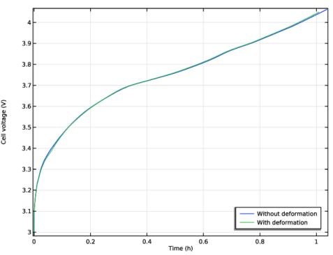
1
|
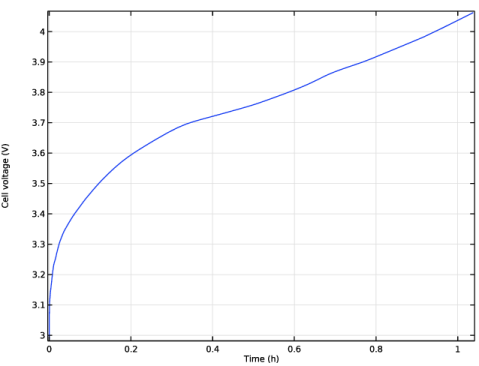
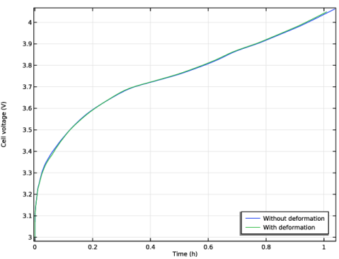
In the Model Builder window, expand the Results > Cell Voltage vs. Time node, then click Cell Voltage vs. Time.
|
|
2
|
|
3
|
Select the Show legends checkbox.
|
|
1
|
|
2
|
|
3
|
|
1
|
|
2
|
|
3
|
|
1
|
|
2
|
|
3
|
|
4
|
|
1
|
In the Model Builder window, expand the Results > Datasets node, then click Study 2 - Full Model/Remeshed Solution 1 (sol5).
|
|
2
|
|
3
|
|
1
|
|
2
|
|
3
|
|
4
|
|
5
|
|
6
|
|
7
|
|
8
|
|
9
|
|
10
|
Clear the Plot dataset edges checkbox.
|
|
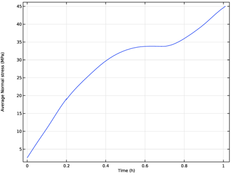
1
|
|
2
|
In the Settings window for 1D Plot Group, type Current Collector Normal Stress vs. Time in the Label text field.
|
|
3
|
Locate the Plot Settings section.
|
|
4
|
|
5
|
|
6
|
|
1
|
|
2
|
|
3
|
|
4
|
|
5
|