PDF

Vibrating Micromirror with Viscous and Thermal Damping
Introduction
Micromirror systems are part of small MEMS (microelectromechanical systems) systems for integrated scanning micromirror systems in telecommunications and consumer applications. The mirrors have low power consumption and the manufacturing cost is low. Their applications range from microscopy applications, medical imaging, scanners, and heads-up displays, to some fiber optics applications.
Figure 1: Geometry of the micromirror system including the fixed constraint, the torquing force components F, and the symmetry plane.
The dynamic vibrating behavior of the micromirror (or other MEMS resonators) and especially the damping is an important factor affecting the design of their actuator systems. In the development process of new micromirror systems, modeling the damping correctly, and thus predicting the performance of the system, can save both time and money.
This model presents a highly simplified micromirror geometry modeled with the Shell physics interface coupled to Thermoviscous Acoustics, Frequency Domain. The model compares the simulated damped vibration results to a simple oscillator model tuned using the results of an eigenfrequency study. For a more advanced micromirror model see the Prestressed Micromirror Vibrations: Thermoviscous–Thermoelasticity Coupling tutorial model also found in the Application Library.
Model Definition
A sketch of the idealized micromirror system modeled here is shown in Figure 1. The mirror is made of silicon and is surrounded by air. It is 0.5 mm by 0.5 mm (only half is shown in the figure because of symmetry) and has a thickness of 1 μm.
The solid mirror is modeled using shell elements and the surrounding air is modeled using thermoviscous acoustics. A pressure acoustics layer is used to truncate the computational domain. The model combines the Shell interface, the Thermoviscous Acoustics, Frequency Domain interface, and the Pressure Acoustics, Frequency Domain interface. The three physics interfaces are set up and combined using multiphysics couplings: the Acoustic–Thermoviscous Acoustics Boundary and the Thermoviscous Acoustic–Structure Boundary.
One goal with the model is to get a correct assessment of the damping the mirror experiences. Therefore, the detailed thermoviscous acoustics is used to model the air domain surrounding the micromirror. The interface includes thermal and viscous damping explicitly as it solves the full linearized Navier–Stokes, continuity, and energy equations, implemented in the Thermoviscous Acoustics, Frequency Domain interface.
An important parameter in such models is the thickness of the viscous and thermal boundary layers (also called the penetration depths). It is in these layers that the energy is dissipated (viscous drag and thermal conduction). For air, the layers are of approximately the same size. The thickness of the viscous boundary layer δv is given by the expression
(1)
since δv = 0.22 mm at 100 Hz. The boundary layer thickness can also be evaluated in postprocessing through the variables tash.d_visc and tash.d_therm.
The model is both solved using a frequency-domain sweep and using an eigenfrequency study. The frequency sweep results in a frequency response where the displacement (or velocity) is evaluated at the tip of the mirror (on the symmetry plane).
The response at the resonance yields the Q-factor Qr and the resonance frequency fr. Their expected values are computed based on the eigenfrequency analysis results. The Q-factor is defined as
where f0 is the resonance frequency and Δf is the peak width at half power (which corresponds to the 3 dB down width). The value of the band width is evaluated in the results using the Graph Marker functionality, see Figure 7 (bottom). The Q-factor is related to the attenuation rate α through
The result of the eigenfrequency study is a complex-valued eigenfrequency fc which relates to the other parameters through
(2)
Finally, the response of an underdamped harmonic oscillator can be written as
(3)
where F is the actuating force and v is the velocity of the oscillator. This expression is used as a model equation for the frequency response in the vicinity of the resonance frequency, based on parameters identified in the eigenfrequency analysis (using the relations in Equation 2).
Results and Discussion
The first two modes from the eigenfrequency study are shown in Figure 2. The torquing mode studied in the subsequent frequency domain analysis is the top figure where fc is at about 10.5 kHz, while a symmetric vibrating mode is found at about 13 kHz. The next mode (not shown) is at nearly 40 kHz. The modal von Mises stress for the first mode is shown in Figure 3. It is important to note the regions of high stress, these are also the regions where a finer mesh needs to be used to capture the full dynamics.
Figure 2: Displacement plot of the torquing (top) and symmetric (bottom) vibrating modes of the micromirror.
Figure 3: Von Mises stress distribution in the shell for first (torquing) mode.
The displacement of the micromirror with the torquing actuation is shown in Figure 4 at a frequency of 10 kHz. The acoustic temperature variations and the acoustic pressure distribution also at 10 kHz is shown in Figure 5. The instantaneous local velocity (acoustic variations in the velocity) is shown in Figure 6. A high velocity region is seen near the edge of the micromirror. The extent of this region into the surrounding air is given by the scale of the viscous boundary layer (also known as the viscous penetration depth, Equation 1). The thermal boundary layer (thermal penetration depth) can in the same way be identified in Figure 5 (top).
The displacement response of the system is plotted in Figure 7 (top). This plot shows the absolute value of the z-component of the displacement field |wshell| evaluated at the tip of the micromirror. The bottom part of this figure shows the power response, on the dB scale (normalized by the maximum), by plotting
and comparing to the model expression given in Equation 3. The parameters used in the analytical model expression stem from the eigenfrequency derived in the eigenfrequency study. The value of the eigenfrequency fc and the other parameters used in the analytical model are defined as variables (see the Component 1 > Definitions > Variables 1). The values of the variables evaluated for the first eigenfrequency, are computed in the Evaluation Group in the model. Using the computed value leads to good agreement between the two power response curves, as seen in Figure 7 (bottom). The figure also shows the bandwidth of the frequency response, this value agrees well with the value extracted from the eigenfrequency analysis and evaluated in the Evaluation Group.
Figure 4: Displacement of the micromirror at 10 kHz subject to the torquing force.
Figure 5: (top) Temperature field in the thermoviscous acoustics domain around the micromirror, and (bottom) pressure isosurfaces showing the antisymmetric pressure distribution.
Figure 6: The instantaneous local velocity, with clear high velocity regions near the mirror edges. The extent of the high velocity region is given by the scale of the acoustic viscous boundary layer.
Figure 7: (top) Displacement response, and (bottom) power response with half-power bandwidth and analytical model curve.
Application Library path: Acoustics_Module/Vibrations_and_FSI/vibrating_micromirror
Modeling Instructions
From the File menu, choose New.
New
In the New window, click  Model Wizard.
Model Wizard
1
In the Model Wizard window, click  3D.
2
In the Select Physics tree, select Structural Mechanics > Shell (shell).
3
Click Add.
4
In the Select Physics tree, select Acoustics > Thermoviscous Acoustics > Thermoviscous Acoustics, Frequency Domain (ta).
5
Click Add.
6
In the Select Physics tree, select Acoustics > Pressure Acoustics > Pressure Acoustics, Frequency Domain (acpr).
7
Click Add.
8
Click  Study.
9
In the Select Study tree, select General Studies > Eigenfrequency.
10
Global Definitions
Parameters 1
1
In the Model Builder window, under Global Definitions click Parameters 1.
2
In the Settings window for Parameters, locate the Parameters section.
3
Click  Load from File.
4
Geometry 1
The geometry sequence for the model (see Figure 1) is available in a file. If you want to create it from scratch yourself, you can follow the instructions in the Appendix — Geometry Modeling Instructions section. Otherwise, insert the geometry sequence as follows:
1
In the Geometry toolbar, click Insert Sequence and choose Insert Sequence.
2
3
In the Geometry toolbar, click  Build All.
4
Click the  Go to Default View button in the Graphics toolbar.
5
Click the  Wireframe Rendering button in the Graphics toolbar.
Definitions
Variables 1
1
In the Model Builder window, under Component 1 (comp1) right-click Definitions and choose Variables.
2
In the Settings window for Variables, locate the Variables section.
3
Click  Load from File.
4
Shell
1
In the Definitions toolbar, click  Explicit.
2
In the Settings window for Explicit, type Shell in the Label text field.
3
Locate the Input Entities section. From the Geometric entity level list, choose Boundary.
4
Symmetry
1
In the Definitions toolbar, click  Explicit.
2
In the Settings window for Explicit, type Symmetry in the Label text field.
3
Locate the Input Entities section. From the Geometric entity level list, choose Boundary.
4
Symmetry Edge
1
In the Definitions toolbar, click  Explicit.
2
In the Settings window for Explicit, type Symmetry Edge in the Label text field.
3
Locate the Input Entities section. From the Geometric entity level list, choose Edge.
4
Add Material
1
In the Materials toolbar, click  Add Material to open the Add Material window.
2
Go to the Add Material window.
3
In the tree, select Built-in > Air.
4
Click the Add to Component button in the window toolbar.
5
In the tree, select Built-in > Silicon.
6
Click the Add to Component button in the window toolbar.
7
In the Materials toolbar, click  Add Material to close the Add Material window.
Materials
Silicon (mat2)
1
In the Settings window for Material, locate the Geometric Entity Selection section.
2
From the Geometric entity level list, choose Boundary.
3
From the Selection list, choose Shell.
Shell (shell)
1
In the Model Builder window, under Component 1 (comp1) click Shell (shell).
2
In the Settings window for Shell, locate the Boundary Selection section.
3
From the Selection list, choose Shell.
Thickness and Offset 1
1
In the Model Builder window, under Component 1 (comp1) > Shell (shell) click Thickness and Offset 1.
2
In the Settings window for Thickness and Offset, locate the Thickness and Offset section.
3
In the d0 text field, type h_mirror.
Fixed Constraint 1
1
In the Physics toolbar, click  Edges and choose Fixed Constraint.
2
Symmetry 1
1
In the Physics toolbar, click  Edges and choose Symmetry.
2
In the Settings window for Symmetry, locate the Edge Selection section.
3
From the Selection list, choose Symmetry Edge.
Body Load 1
1
In the Physics toolbar, click  Boundaries and choose Body Load.
2
In the Settings window for Body Load, locate the Boundary Selection section.
3
From the Selection list, choose Shell.
4
Locate the Force section. Specify the fV vector as
This corresponds to a torquing force proportional to the x-coordinate acting in the z direction. A load of 0 N/m3 act in the middle (at x = 0) rising to 1e5 N/m3 at the mirror edge.
Thermoviscous Acoustics, Frequency Domain (ta)
1
In the Model Builder window, under Component 1 (comp1) click Thermoviscous Acoustics, Frequency Domain (ta).
2
In the Settings window for Thermoviscous Acoustics, Frequency Domain, locate the Domain Selection section.
3
Click  Clear Selection.
4
Symmetry 1
1
In the Physics toolbar, click  Boundaries and choose Symmetry.
2
In the Settings window for Symmetry, locate the Boundary Selection section.
3
From the Selection list, choose Symmetry.
Pressure Acoustics, Frequency Domain (acpr)
1
In the Model Builder window, under Component 1 (comp1) click Pressure Acoustics, Frequency Domain (acpr).
2
3
In the Physics toolbar, click  Boundaries and choose Symmetry.
1
In the Settings window for Symmetry, locate the Boundary Selection section.
2
From the Selection list, choose Symmetry.
Spherical Wave Radiation 1
1
In the Physics toolbar, click  Boundaries and choose Spherical Wave Radiation.
2
Proceed to set up the Multiphysics couplings that couple Thermoviscous Acoustics to Pressure Acoustics and couple the interior shell to the surrounding thermoviscous acoustics domain.
Multiphysics
Acoustic–Thermoviscous Acoustic Boundary 1 (atb1)
1
In the Physics toolbar, click  Multiphysics Couplings and choose Boundary > Acoustic–Thermoviscous Acoustic Boundary.
2
In the Settings window for Acoustic–Thermoviscous Acoustic Boundary, locate the Boundary Selection section.
3
From the Selection list, choose All boundaries.
When you select All boundaries COMSOL automatically detects where a thermoviscous acoustics domain and a pressure acoustics domain meet and applies the coupling there.
Thermoviscous Acoustic–Structure Boundary 1 (tsb1)
1
In the Physics toolbar, click  Multiphysics Couplings and choose Boundary > Thermoviscous Acoustic–Structure Boundary.
2
In the Settings window for Thermoviscous Acoustic–Structure Boundary, locate the Boundary Selection section.
3
From the Selection list, choose Shell.
Selecting All boundaries here will result in the same setup as using the Shell selection.
Mesh 1
Free Triangular 1
1
In the Mesh toolbar, click  More Generators and choose Free Triangular.
2
In the Settings window for Free Triangular, locate the Boundary Selection section.
3
From the Selection list, choose Shell.
Size 1
1
Right-click Free Triangular 1 and choose Size.
2
In the Settings window for Size, locate the Element Size section.
3
Click the Custom button.
4
Locate the Element Size Parameters section.
5
Select the Maximum element size checkbox. In the associated text field, type 0.8*dvisc.
To get a fully resolved acoustic boundary layer, it is also necessary to add a boundary layer mesh. Do this as the last mesh step.
6
Select the Minimum element size checkbox. In the associated text field, type 0.1*dvisc.
7
Select the Maximum element growth rate checkbox. In the associated text field, type 1.4.
8
Select the Curvature factor checkbox. In the associated text field, type 0.4.
Size 2
1
In the Model Builder window, right-click Free Triangular 1 and choose Size.
2
In the Settings window for Size, locate the Geometric Entity Selection section.
3
From the Geometric entity level list, choose Point.
4
5
Locate the Element Size section. Click the Custom button.
6
Locate the Element Size Parameters section.
7
Select the Maximum element size checkbox. In the associated text field, type 0.2*dvisc.
Size 3
1
Right-click Free Triangular 1 and choose Size.
2
In the Settings window for Size, locate the Geometric Entity Selection section.
3
From the Geometric entity level list, choose Edge.
4
5
Locate the Element Size section. Click the Custom button.
6
Locate the Element Size Parameters section.
7
Select the Maximum element size checkbox. In the associated text field, type 0.5*dvisc.
8
Click  Build Selected.
The surface mesh of the mirror should look like this. Notice the higher mesh resolution regions. As seen in results, these are the regions with higher stress.
Size
1
In the Model Builder window, under Component 1 (comp1) > Mesh 1 click Size.
2
In the Settings window for Size, locate the Element Size section.
3
Click the Custom button.
4
Locate the Element Size Parameters section. In the Maximum element size text field, type 343[m/s]/f0/6.
5
In the Resolution of narrow regions text field, type 2.
Free Tetrahedral 1
In the Mesh toolbar, click  Free Tetrahedral.
Boundary Layers 1
In the Mesh toolbar, click  Boundary Layers.
Boundary Layer Properties
1
In the Model Builder window, click Boundary Layer Properties.
2
In the Settings window for Boundary Layer Properties, locate the Geometric Entity Selection section.
3
From the Selection list, choose Shell.
4
Locate the Layers section. In the Number of layers text field, type 3.
5
From the Thickness specification list, choose First layer.
6
In the Thickness text field, type 0.3*dvisc.
7
Click  Build All.
The geometry with mesh should look like the figure below.
Proceed with the eigenfrequency study. The determined eigenfrequency including the complex part yields information about the attenuation in the system.
Study 1
Step 1: Eigenfrequency
1
In the Model Builder window, under Study 1 click Step 1: Eigenfrequency.
2
In the Settings window for Eigenfrequency, locate the Study Settings section.
3
In the Search for eigenfrequencies around shift text field, type 10000.
4
From the Search method around shift list, choose Larger real part.
5
Select the Desired number of eigenfrequencies checkbox. In the associated text field, type 3.
These selections will search for the first three eigenmodes above 10 kHz. It is known that the first eigenfrequency is at about 10500 Hz (this can also be determined using a frequency study looking for the response peaks). The eigenfrequency search condition will make the solution converge faster. Selecting the Closest in absolute value will search for modes with both smaller and larger eigenfrequencies.
Again, turn off the generation of the default plots and generate and show the default solver to take a look at the solver suggestions.
6
In the Model Builder window, click Study 1.
7
In the Settings window for Study, locate the Study Settings section.
8
Clear the Generate default plots checkbox.
Solution 1 (sol1)
1
In the Study toolbar, click  Show Default Solver.
2
In the Model Builder window, expand the Solution 1 (sol1) node.
Select and enable the first suggested iterative solver. In the eigenfrequency study for this size of problem, the direct solver is faster but it is more memory consuming.
3
In the Model Builder window, expand the Study 1 > Solver Configurations > Solution 1 (sol1) > Eigenvalue Solver 1 node.
4
Right-click Study 1 > Solver Configurations > Solution 1 (sol1) > Eigenvalue Solver 1 > Suggested Iterative Solver (GMRES with Direct Precond.) (tsb1_atb1) and choose Enable.
5
In the Study toolbar, click  Compute.
Result Templates
1
In the Results toolbar, click  Result Templates to open the Result Templates window.
2
Go to the Result Templates window.
3
In the tree, select Study 1/Solution 1 (sol1) > Shell > Mode Shape (shell).
4
Click the Add Result Template button in the window toolbar.
5
In the Results toolbar, click  Result Templates to close the Result Templates window.
Results
Mode Shape (shell)
1
Click the  Zoom Extents button in the Graphics toolbar.
The default (first) selected eigenvalue is the vibrating torque mode at about 10,500 Hz. This is the vibration mode that will be studied next in the frequency domain study.
The first mode should look like the one in Figure 2 top.
The next eigenmode represents a symmetric vibration in the transverse direction happening at about 13100 Hz.
2
In the Settings window for 3D Plot Group, locate the Data section.
3
From the Eigenfrequency (Hz) list, choose 13068+165.21i.
4
In the Mode Shape (shell) toolbar, click  Plot.
The second mode should look like the one in Figure 2 bottom.
The next mode happens at nearly 40 kHz and can be seen by selecting the last of the three computed eigenfrequencies.
Result Templates
1
In the Results toolbar, click  Result Templates to open the Result Templates window.
2
Go to the Result Templates window.
3
In the tree, select Study 1/Solution 1 (sol1) > Shell > Modal Stress (shell).
4
Click the Add Result Template button in the window toolbar.
5
In the Results toolbar, click  Result Templates to close the Result Templates window.
Results
Modal Stress (shell)
This second plot shows the von Mises stress distribution in the shell. To further improve the precision of the computed eigenfrequency, the mesh can be refined in the high-stress regions. Note that refining the mesh will rapidly lead to an increased computational time and memory consumption when solving.
Add Study
1
In the Home toolbar, click  Add Study to open the Add Study window.
2
Go to the Add Study window.
3
Find the Studies subsection. In the Select Study tree, select General Studies > Frequency Domain.
4
Click the Add Study button in the window toolbar.
5
In the Home toolbar, click  Add Study to close the Add Study window.
Study 2
Step 1: Frequency Domain
1
In the Settings window for Frequency Domain, locate the Study Settings section.
2
In the Frequencies text field, type range(f0-deltaf,50,f0+deltaf).
Turn off the generation of default plots, only create the ones you need or use the Result Templates. Plot the acoustic variations in temperature, pressure, and velocity as well as response curves. If turned on, the default plots for each physics interface will be generated.
3
In the Model Builder window, click Study 2.
4
In the Settings window for Study, locate the Study Settings section.
5
Clear the Generate default plots checkbox.
Now, generate and show the default solver to take a look at the solver suggestions automatically generated.
Solution 2 (sol2)
1
In the Study toolbar, click  Show Default Solver.
2
In the Model Builder window, expand the Solution 2 (sol2) node.
In this model, which couples pressure acoustics, thermoviscous acoustics, and shell, the default solver is a direct solver. Select and enable the first iterative suggestion. It is faster and more memory efficient than the direct solver.
3
In the Model Builder window, expand the Study 2 > Solver Configurations > Solution 2 (sol2) > Stationary Solver 1 node.
4
Right-click Study 2 > Solver Configurations > Solution 2 (sol2) > Stationary Solver 1 > Suggested Iterative Solver (GMRES with Direct Precond.) (tsb1_atb1) and choose Enable.
5
In the Study toolbar, click  Compute.
Results
In the Model Builder window, expand the Results node.
Mirror 3D 1
1
In the Model Builder window, expand the Results > Datasets node.
2
Right-click Results > Datasets and choose More 3D Datasets > Mirror 3D.
3
In the Settings window for Mirror 3D, locate the Plane Data section.
4
From the Plane list, choose XZ-planes.
5
Locate the Data section. From the Dataset list, choose Study 2/Solution 2 (sol2).
Displacement
1
In the Results toolbar, click  3D Plot Group.
2
In the Settings window for 3D Plot Group, type Displacement in the Label text field.
3
Locate the Data section. From the Dataset list, choose Mirror 3D 1.
Surface 1
1
Right-click Displacement and choose Surface.
2
In the Settings window for Surface, locate the Expression section.
3
From the Unit list, choose µm.
4
Locate the Coloring and Style section. From the Color table list, choose SpectrumLight.
Deformation 1
Right-click Surface 1 and choose Deformation.
Displacement
1
In the Settings window for 3D Plot Group, locate the Data section.
2
From the Parameter value (freq (Hz)) list, choose 10000.
3
Locate the Color Legend section. Select the Show units checkbox.
4
In the Displacement toolbar, click  Plot.
The plot should look like the one in Figure 4.
Temperature Variation
1
In the Results toolbar, click  3D Plot Group.
2
In the Settings window for 3D Plot Group, type Temperature Variation in the Label text field.
3
Locate the Data section. From the Dataset list, choose Study 2/Solution 2 (sol2).
4
Locate the Color Legend section. Select the Show units checkbox.
Slice 1
1
Right-click Temperature Variation and choose Slice.
2
In the Settings window for Slice, locate the Expression section.
3
In the Expression text field, type ta.T_t.
4
From the Unit list, choose mK.
5
Locate the Plane Data section. From the Plane list, choose ZX-planes.
6
Locate the Coloring and Style section. From the Color table list, choose ThermalWave.
7
From the Scale list, choose Linear symmetric.
8
In the Temperature Variation toolbar, click  Plot.
The plot should look like the one in Figure 5 top.
Acoustic Pressure
1
In the Results toolbar, click  3D Plot Group.
2
In the Settings window for 3D Plot Group, type Acoustic Pressure in the Label text field.
3
Locate the Data section. From the Dataset list, choose Study 2/Solution 2 (sol2).
4
Locate the Color Legend section. Select the Show units checkbox.
Isosurface 1
1
Right-click Acoustic Pressure and choose Isosurface.
2
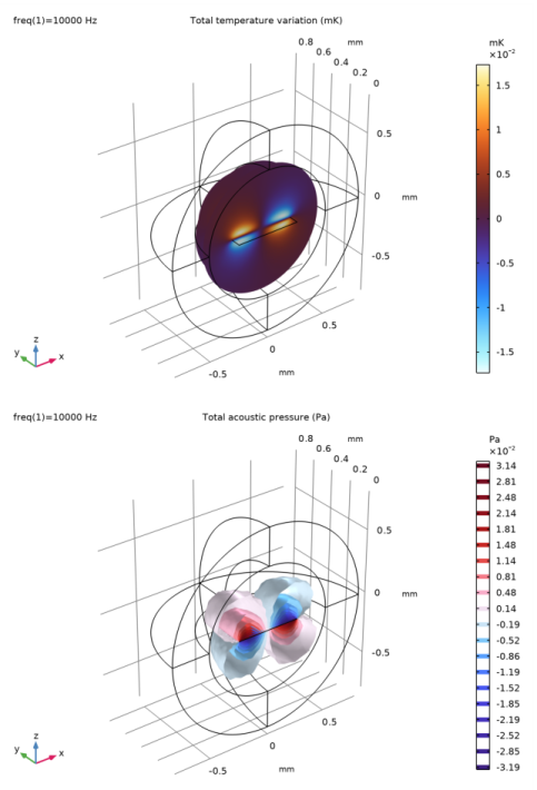
In the Settings window for Isosurface, click Replace Expression in the upper-right corner of the Expression section. From the menu, choose Component 1 (comp1) > Multiphysics > atb1.p_t - Total acoustic pressure - Pa.
3
Locate the Levels section. In the Total levels text field, type 20.
4
Locate the Coloring and Style section. From the Color table list, choose Wave.
5
From the Scale list, choose Linear symmetric.
6
In the Acoustic Pressure toolbar, click  Plot.
The plot should look like the one in Figure 5 bottom.
Acoustic Velocity
1
In the Model Builder window, right-click Temperature Variation and choose Duplicate.
2
In the Settings window for 3D Plot Group, type Acoustic Velocity in the Label text field.
3
Locate the Data section. From the Dataset list, choose Study 2/Solution 2 (sol2).
4
Locate the Color Legend section. Select the Show units checkbox.
Slice 1
1
In the Model Builder window, expand the Acoustic Velocity node, then click Slice 1.
2
In the Settings window for Slice, locate the Expression section.
3
In the Expression text field, type ta.v_inst.
4
From the Unit list, choose mm/s.
5
Locate the Coloring and Style section. From the Color table list, choose Rainbow.
6
From the Scale list, choose Linear.
7
In the Acoustic Velocity toolbar, click  Plot.
The plot should look like the one in Figure 6.
Proceed to setting up two 1D curves that represent the frequency response of the system by probing the displacement at the symmetry plane of the micromirror. The first plot gives the absolute value of the displacement. The second plot depicts the power (proportional to the velocity squared) on the dB scale and compared to a simple harmonic oscillator model tuned using parameters extracted from an eigenfrequency study of the system (instructions follow below). The parameters are given in the parameters list. Both curves are normalized by the maximum value.
Displacement Response
1
In the Results toolbar, click  1D Plot Group.
2
In the Settings window for 1D Plot Group, type Displacement Response in the Label text field.
3
Locate the Data section. From the Dataset list, choose Study 2/Solution 2 (sol2).
4
Click to expand the Title section. From the Title type list, choose Label.
Point Graph 1
1
Right-click Displacement Response and choose Point Graph.
2
3
In the Settings window for Point Graph, locate the y-Axis Data section.
4
In the Expression text field, type abs(w).
5
In the Displacement Response toolbar, click  Plot.
The plot should look like the one in Figure 7 top. Proceed and create a plot to compare the simple resonator expression with the actual response of the system.
Power Response
1
In the Results toolbar, click  1D Plot Group.
2
In the Settings window for 1D Plot Group, type Power Response in the Label text field.
3
Locate the Data section. From the Dataset list, choose Study 2/Solution 2 (sol2).
4
Click to expand the Title section. From the Title type list, choose Label.
5
Locate the Legend section. From the Position list, choose Lower left.
Point Graph 1
1
Right-click Power Response and choose Point Graph.
2
3
In the Settings window for Point Graph, locate the y-Axis Data section.
4
In the Expression text field, type 20*log10(abs(w*ta.iomega))-with(12,20*log10(abs(w*ta.iomega))).
5
Click to expand the Legends section. Select the Show legends checkbox.
6
From the Legends list, choose Manual.
7
Global 1
1
In the Model Builder window, right-click Power Response and choose Global.
2
In the Settings window for Global, locate the y-Axis Data section.
3
Graph Marker 1
1
In the Model Builder window, right-click Point Graph 1 and choose Graph Marker.
2
In the Settings window for Graph Marker, locate the Display section.
3
From the Display mode list, choose Bandwidth.
4
From the Cutoff mode list, choose Offset from peak.
5
Locate the Text Format section. In the Precision text field, type 5.
6
Select the Include unit checkbox.
7
In the Power Response toolbar, click  Plot.
The plot should look like the one in Figure 7 bottom. Finally, add an evaluation group to evaluate the harmonic oscillator parameters used in the simple analytical model.
Evaluation Group 1 - Harmonic Oscillator Parameters
1
In the Results toolbar, click  Evaluation Group.
2
In the Settings window for Evaluation Group, locate the Data section.
3
From the Eigenfrequency selection list, choose First.
4
In the Label text field, type Evaluation Group 1 - Harmonic Oscillator Parameters.
5
Locate the Transformation section. Select the Transpose checkbox.
Global Evaluation 1
1
Right-click Evaluation Group 1 - Harmonic Oscillator Parameters and choose Global Evaluation.
2
In the Settings window for Global Evaluation, locate the Expressions section.
3
4
In the Evaluation Group 1 - Harmonic Oscillator Parameters toolbar, click  Evaluate.
Appendix — Geometry Modeling Instructions
If you want to create the geometry yourself, follow these steps.
Geometry 1
1
In the Model Builder window, under Component 1 (comp1) click Geometry 1.
2
In the Settings window for Geometry, locate the Units section.
3
From the Length unit list, choose mm.
Work Plane 1 (wp1)
1
In the Geometry toolbar, click  Work Plane.
2
In the Settings window for Work Plane, click  Go to Plane Geometry.
Work Plane 1 (wp1) > Plane Geometry
In the Model Builder window, click Plane Geometry.
Work Plane 1 (wp1) > Rectangle 1 (r1)
1
In the Work Plane toolbar, click  Rectangle.
2
In the Settings window for Rectangle, locate the Size and Shape section.
3
In the Width text field, type 0.5.
4
In the Height text field, type 0.5.
5
Locate the Position section. From the Base list, choose Center.
Work Plane 1 (wp1) > Rectangle 2 (r2)
1
In the Work Plane toolbar, click  Rectangle.
2
In the Settings window for Rectangle, locate the Size and Shape section.
3
In the Width text field, type 0.1.
4
In the Height text field, type 0.05.
5
Locate the Position section. In the xw text field, type -0.05.
6
In the yw text field, type 0.25.
Work Plane 1 (wp1) > Rectangle 3 (r3)
1
Right-click Component 1 (comp1) > Geometry 1 > Work Plane 1 (wp1) > Plane Geometry > Rectangle 2 (r2) and choose Duplicate.
2
In the Settings window for Rectangle, locate the Position section.
3
In the yw text field, type -0.3.
Work Plane 1 (wp1) > Rectangle 4 (r4)
1
In the Work Plane toolbar, click  Rectangle.
2
In the Settings window for Rectangle, locate the Size and Shape section.
3
In the Width text field, type 0.5.
4
In the Height text field, type 0.6.
5
Locate the Position section. From the Base list, choose Center.
6
Right-click Rectangle 4 (r4) and choose Build All Objects.
Work Plane 1 (wp1) > Union 1 (uni1)
1
In the Work Plane toolbar, click  Booleans and Partitions and choose Union.
2
Click the  Select All button in the Graphics toolbar.
3
In the Settings window for Union, click  Build Selected.
Work Plane 1 (wp1) > Delete Entities 1 (del1)
1
In the Model Builder window, right-click Plane Geometry and choose Delete Entities.
2
On the object uni1, select Boundaries 1, 2, 5, 7, 10, 12, 15, 19, 20, and 22 only.
3
In the Settings window for Delete Entities, click  Build Selected.
Work Plane 1 (wp1) > Fillet 1 (fil1)
1
In the Work Plane toolbar, click  Fillet.
2
On the object del1, select Points 4, 5, 8, and 9 only.
3
In the Settings window for Fillet, locate the Radius section.
4
In the Radius text field, type 0.01.
5
Click  Build Selected.
Sphere 1 (sph1)
1
In the Model Builder window, right-click Geometry 1 and choose Sphere.
2
In the Settings window for Sphere, locate the Size section.
3
In the Radius text field, type 0.8.
4
Click to expand the Layers section. In the table, enter the following settings:
Union 1 (uni1)
1
In the Geometry toolbar, click  Booleans and Partitions and choose Union.
To better see the entire geometry use the Zoom Extents tool.
2
Click in the Graphics window and then press Ctrl+A to select both objects.
3
In the Settings window for Union, click  Build Selected.
Block 1 (blk1)
1
In the Geometry toolbar, click  Block.
2
In the Settings window for Block, locate the Size and Shape section.
3
In the Width text field, type 2.
4
In the Depth text field, type 2.
5
In the Height text field, type 2.
6
Locate the Position section. From the Base list, choose Center.
7
In the y text field, type -1.
8
Click  Build Selected.
Difference 1 (dif1)
1
In the Geometry toolbar, click  Booleans and Partitions and choose Difference.
2
3
In the Settings window for Difference, locate the Difference section.
4
Click to select the  Activate Selection toggle button for Objects to subtract.
5
6
Click  Build All Objects.