PDF

Type 4.3 Ear Simulator
Introduction
This model is of the P.57 Type 4.3 Full-Band Ear Simulator. The model includes the geometry of the ear canal as well as the pinna defined in the ITU-T P.57 standard. The model also includes interpolation data for an ear drum impedance ensuring correct acoustic properties of the ear. The model tries to fulfill the geometry and acoustic requirements defined in the standard. It is not a model of a particular, commercially available, ear simulator.
Model Definition
This model imports a geometry representation of the ear canal (Figure 1) as well as the combined pinna and ear canal (Figure 2) that is defined in the ITU-T P.57 standard, Ref. 1. To fulfill the acoustic requirements specified in the ITU-T P.57 standard, the eardrum impedance presented in Nielsen and Jensen, 2022 (Ref. 2) is imported as an interpolation function and used. Some details about the construction of the geometry are presented in Ref. 2.
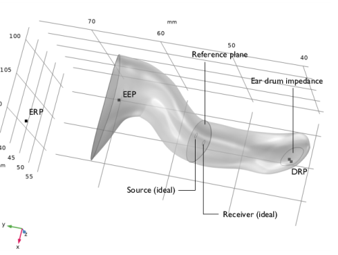
Figure 1: Geometry of the ear canal including reference plane.
A typical use case, where an in-ear device is tested (for example, a hearing aid) in the artificial ear, is presented in Nielsen and Jensen, 2023 (Ref. 3). In the reference, a comparison between measurements (using a commercially available ear simulator) and simulations using the present ear geometry and impedance is carried out. The presented results show good correlation.
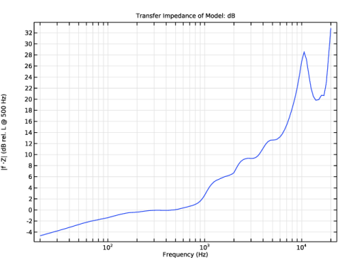
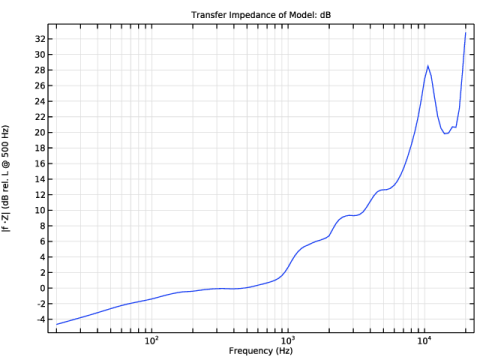
In the first model component (Component 1), the ear canal geometry shown in Figure 1 is imported. The image shows the ear reference point (ERP, here outside of the geometry), the ear entrance point (EEP), and the eardrum reference point (EDP). The image also shows the reference plane which is used when defining the transfer impedance of the system. A simulation, mimicking a typical measurement setup to compute the transfer impedance from the reference plane to the eardrum, is set up. The transfer impedance (absolute value of) is the acoustic characteristic defined in the ITU-T P.57 standard. The resulting absolute valued transfer impedance (times the frequency) |Z·f| is depicted in the results section in Figure 4. A comparison between a simulated transfer impedance and the standard is shown in Ref. 1. The location of an ideal source and an ideal receiver (corresponding to probes tubes in a typical measurement) is also depicted in Figure 1.
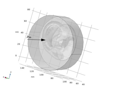
Figure 2: Geometry of the combined ear canal and pinna, including an exterior cylindrical air domain.
In the second model component (Component 2), the combined ear canal and pinna shown in Figure 2 is imported. The geometry also includes an exterior cylindrical air domain. Using this geometry, the open ear response to a normally incident plane wave pin is simulated (see the arrow in Figure 2). The open boundaries of the cylindrical air domain are modeled using the Perfectly Matched Boundary condition.
Results and Discussion
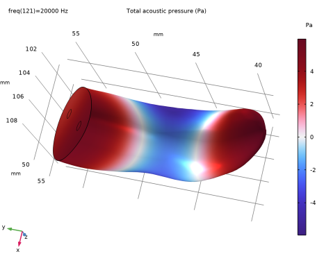
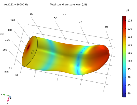
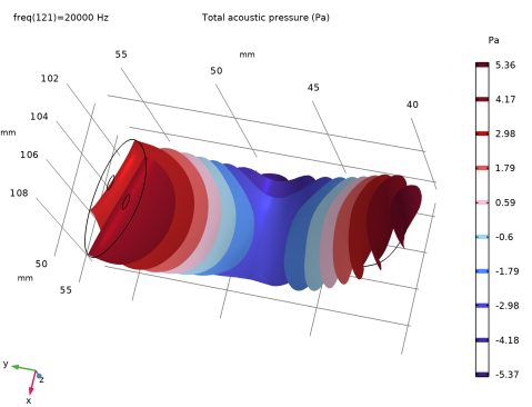
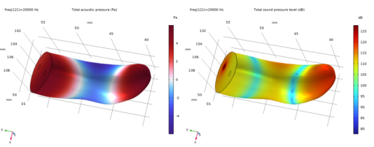
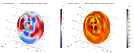
The pressure and sound pressure level (SPL) distributions in the ear canal (from the reference plane to the ear drum) evaluated at 20 kHz are depicted in Figure 3. The absolute value of the transfer impedance (times the frequency) |Z·f| is depicted in Figure 4. This curve represents the acoustic signature of the ear simulator described in the ITU-T P.57 standard.
Figure 3: Pressure (left) and SPL (right) distribution in the ear canal at 20 kHz.
Figure 4: Absolute value of the transfer impedance (times frequency) as function of frequency. Computed from the reference plane to the ear drum.
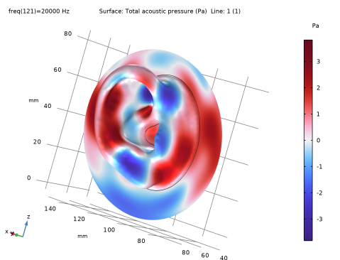
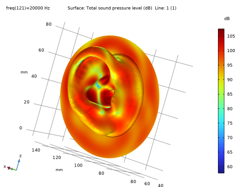
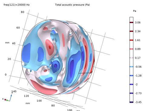
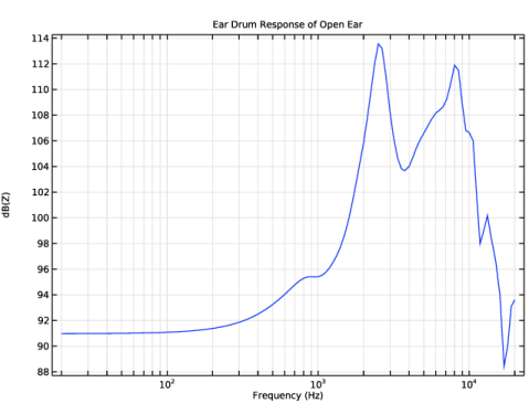
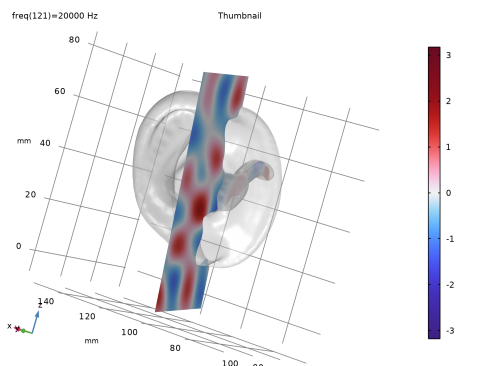
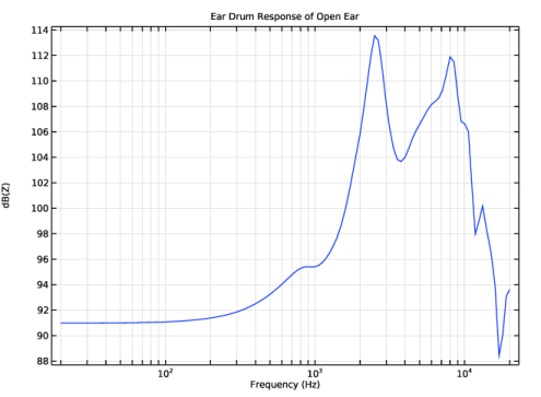
The total pressure (incident plus scattered) and the total SPL at the surface of the pinna for the setup described in Figure 2 is depicted in Figure 5. The open ear response as a function of frequency is depicted in Figure 6; here specifically showing the sound pressure level at the ear drum.
Figure 5: Total pressure (left) and SPL (right) distribution on the surface of the ear at 20 kHz.
Figure 6: Ear drum response of the open ear as function of frequency.
References
1. ITU-T Recommendation P.57: Artificial Ears. 2021.
2. L.B. Nielsen and M. Herring Jensen, “The Digital Twin of a New and Standardized Fullband Ear Simulator,” DAGA 2022.
3. L.B. Nielsen and M. Herring Jensen, “Simulation and physical testing using standardized ear simulator,” DAGA 2023.
Application Library path: Acoustics_Module/Tutorials,_Thermoviscous_Acoustics/type_43_ear_simulator
Modeling Instructions
From the File menu, choose New.
New
In the New window, click  Model Wizard.
Model Wizard
1
In the Model Wizard window, click  3D.
2
In the Select Physics tree, select Acoustics > Pressure Acoustics > Pressure Acoustics, Frequency Domain (acpr).
3
Click Add.
4
Click  Study.
5
In the Select Study tree, select General Studies > Frequency Domain.
6
Global Definitions
Parameters 1
1
In the Model Builder window, under Global Definitions click Parameters 1.
2
In the Settings window for Parameters, locate the Parameters section.
3
Interpolation 1 (int1)
1
In the Home toolbar, click  Functions and choose Global > Interpolation.
2
In the Settings window for Interpolation, locate the Definition section.
3
From the Data source list, choose File.
4
Click  Browse.
5
6
Click  Import.
7
Locate the Data Column Settings section. In the table, click to select the cell at row number 1 and column number 1.
8
In the Unit text field, type 1.
9
10
In the Name text field, type absZ.
11
In the Unit text field, type kg/(m^2*s).
12
13
In the Name text field, type argZ.
14
In the Unit text field, type rad.
15
Locate the Interpolation and Extrapolation section. From the Interpolation list, choose Piecewise cubic.
16
From the Extrapolation list, choose Linear.
Geometry 1
1
In the Model Builder window, under Component 1 (comp1) click Geometry 1.
2
In the Settings window for Geometry, locate the Units section.
3
From the Length unit list, choose mm.
4
Locate the Advanced section. From the Geometry representation list, choose CAD kernel.
Import 1 (imp1)
1
In the Home toolbar, click  Import.
2
In the Settings window for Import, locate the Source section.
3
Click  Browse.
4
5
Click  Import.
6
In the Geometry toolbar, click  Build All.
Ignore Edges 1 (ige1)
1
In the Geometry toolbar, click  Virtual Operations and choose Ignore Edges.
2
On the object fin, select Edges 3, 4, and 17 only.
3
In the Geometry toolbar, click  Build All.
Add Material
1
In the Materials toolbar, click  Add Material to open the Add Material window.
2
Go to the Add Material window.
3
In the tree, select Built-in > Air.
4
Click the Add to Component button in the window toolbar.
5
In the Materials toolbar, click  Add Material to close the Add Material window.
Definitions
Variables 1
1
In the Home toolbar, click  Variables and choose Local Variables.
2
In the Settings window for Variables, locate the Variables section.
3
Source
1
In the Definitions toolbar, click  Explicit.
2
In the Settings window for Explicit, type Source in the Label text field.
3
Locate the Input Entities section. From the Geometric entity level list, choose Boundary.
4
Click  Paste Selection.
5
In the Paste Selection dialog, type 6 in the Selection text field.
6
Probe Microphone
1
In the Definitions toolbar, click  Explicit.
2
In the Settings window for Explicit, type Probe Microphone in the Label text field.
3
Locate the Input Entities section. From the Geometric entity level list, choose Boundary.
4
Click  Paste Selection.
5
In the Paste Selection dialog, type 7 in the Selection text field.
6
Ear Drum
1
In the Definitions toolbar, click  Explicit.
2
In the Settings window for Explicit, type Ear Drum in the Label text field.
3
Locate the Input Entities section. From the Geometric entity level list, choose Boundary.
4
Click  Paste Selection.
5
In the Paste Selection dialog, type 5 in the Selection text field.
6
Integration 1 (intop1)
1
In the Definitions toolbar, click  Nonlocal Couplings and choose Integration.
2
In the Settings window for Integration, locate the Source Selection section.
3
From the Geometric entity level list, choose Boundary.
4
From the Selection list, choose Source.
Average 1 (aveop1)
1
In the Definitions toolbar, click  Nonlocal Couplings and choose Average.
2
In the Settings window for Average, locate the Source Selection section.
3
From the Geometric entity level list, choose Boundary.
4
From the Selection list, choose Ear Drum.
Average 2 (aveop2)
1
In the Definitions toolbar, click  Nonlocal Couplings and choose Average.
2
In the Settings window for Average, locate the Source Selection section.
3
From the Geometric entity level list, choose Boundary.
4
From the Selection list, choose Probe Microphone.
Pressure Acoustics, Frequency Domain (acpr)
1
In the Model Builder window, under Component 1 (comp1) click Pressure Acoustics, Frequency Domain (acpr).
2
In the Settings window for Pressure Acoustics, Frequency Domain, locate the Domain Selection section.
3
Click  Clear Selection.
4
Click  Paste Selection.
5
In the Paste Selection dialog, type 2 in the Selection text field.
6
7
In the Settings window for Pressure Acoustics, Frequency Domain, locate the Typical Wave Speed for Perfectly Matched Layers section.
8
In the cref text field, type 343[m/s].
Impedance 1
1
In the Physics toolbar, click  Boundaries and choose Impedance.
2
In the Settings window for Impedance, locate the Boundary Selection section.
3
From the Selection list, choose Ear Drum.
4
Locate the Impedance section. In the Zn text field, type absZ(log10(freq[1/Hz]))*exp(i*argZ(log10(freq[1/Hz]))).
Normal Velocity 1
1
In the Physics toolbar, click  Boundaries and choose Normal Velocity.
2
In the Settings window for Normal Velocity, locate the Boundary Selection section.
3
From the Selection list, choose Source.
4
Locate the Normal Velocity section. In the vn text field, type vn.
Thermoviscous Boundary Layer Impedance 1
1
In the Physics toolbar, click  Boundaries and choose Thermoviscous Boundary Layer Impedance.
2
In the Settings window for Thermoviscous Boundary Layer Impedance, locate the Boundary Selection section.
3
Click  Paste Selection.
4
In the Paste Selection dialog, type 3 in the Selection text field.
5
6
In the Settings window for Thermoviscous Boundary Layer Impedance, locate the Fluid Properties section.
7
From the Fluid material list, choose Air (mat1).
Mesh
Proceed and generate the mesh using the Physics-controlled mesh functionality. The frequency controlling the maximum element size is per default taken From study. Set the desired Frequencies in the study step. In general, 5 to 6 second-order elements per wavelength are needed to resolve the waves. For more details, see Meshing (Resolving the Waves) in the Acoustics Module User’s Guide. In this model, use the default Automatic option, which gives 5 elements per wavelength.
Add Component
Right-click Thermoviscous Boundary Layer Impedance 1 and choose Add Component > 3D.
Geometry 2
1
In the Settings window for Geometry, locate the Units section.
2
From the Length unit list, choose mm.
Import 1 (imp1)
1
In the Geometry toolbar, click  Import.
2
In the Settings window for Import, locate the Source section.
3
Click  Browse.
4
5
Click  Import.
6
In the Geometry toolbar, click  Build All.
Add Material
1
In the Materials toolbar, click  Add Material to open the Add Material window.
2
Go to the Add Material window.
3
In the tree, select Built-in > Air.
4
Click the Add to Component button in the window toolbar.
5
In the Materials toolbar, click  Add Material to close the Add Material window.
Definitions (comp2)
Ear Drum
1
In the Definitions toolbar, click  Explicit.
2
In the Settings window for Explicit, type Ear Drum in the Label text field.
3
Locate the Input Entities section. From the Geometric entity level list, choose Boundary.
4
Click  Paste Selection.
5
In the Paste Selection dialog, type 8 in the Selection text field.
6
Add Physics
1
In the Home toolbar, click  Add Physics to open the Add Physics window.
2
Go to the Add Physics window.
3
In the tree, select Acoustics > Pressure Acoustics > Pressure Acoustics, Frequency Domain (acpr).
4
Click the Add to Component 2 button in the window toolbar.
5
In the Home toolbar, click  Add Physics to close the Add Physics window.
Pressure Acoustics, Frequency Domain 2 (acpr2)
Thermoviscous Boundary Layer Impedance 1
1
In the Physics toolbar, click  Boundaries and choose Thermoviscous Boundary Layer Impedance.
2
In the Settings window for Thermoviscous Boundary Layer Impedance, locate the Boundary Selection section.
3
Click  Paste Selection.
4
In the Paste Selection dialog, type 6 in the Selection text field.
5
6
In the Settings window for Thermoviscous Boundary Layer Impedance, locate the Fluid Properties section.
7
From the Fluid material list, choose Air (mat2).
Background Pressure Field 1
1
In the Physics toolbar, click  Domains and choose Background Pressure Field.
2
In the Settings window for Background Pressure Field, locate the Domain Selection section.
3
Click  Paste Selection.
4
In the Paste Selection dialog, type 1 in the Selection text field.
5
6
In the Settings window for Background Pressure Field, locate the Background Pressure Field section.
7
In the p0 text field, type 1.
8
From the c list, choose From material.
9
Specify the ek vector as
Perfectly Matched Boundary 1
1
In the Physics toolbar, click  Boundaries and choose Perfectly Matched Boundary.
2
In the Settings window for Perfectly Matched Boundary, locate the Boundary Selection section.
3
Click  Paste Selection.
4
In the Paste Selection dialog, type 1,2,4,7,9 in the Selection text field.
5
6
In the Settings window for Perfectly Matched Boundary, locate the Geometry section.
7
Specify the r0 vector as
Impedance 1
1
In the Physics toolbar, click  Boundaries and choose Impedance.
2
In the Settings window for Impedance, locate the Boundary Selection section.
3
From the Selection list, choose Ear Drum.
4
Locate the Impedance section. In the Zn text field, type absZ(log10(freq[1/Hz]))*exp(i*argZ(log10(freq[1/Hz]))).
Mesh
Proceed and generate the mesh using the Physics-controlled mesh functionality. In this component, use again the default Automatic option, which gives 5 elements per wavelength.
Study 1 - Ear Canal
1
In the Model Builder window, click Study 1.
2
In the Settings window for Study, type Study 1 - Ear Canal in the Label text field.
Step 1: Frequency Domain
1
In the Model Builder window, under Study 1 - Ear Canal click Step 1: Frequency Domain.
2
In the Settings window for Frequency Domain, locate the Study Settings section.
3
Click  Range.
4
In the Range dialog, choose ISO preferred frequencies from the Entry method list.
5
In the Start frequency text field, type 20.
6
In the Stop frequency text field, type 20000.
7
From the Interval list, choose 1/12 octave.
8
Click Add.
9
In the Settings window for Frequency Domain, locate the Physics and Variables Selection section.
10
In the Solve for column of the table, under Component 2 (comp2), clear the checkbox for Pressure Acoustics, Frequency Domain 2 (acpr2).
Solution 1 (sol1)
In the Study toolbar, click  Show Default Solver.
Add Study
1
In the Study toolbar, click  Add Study to open the Add Study window.
2
Go to the Add Study window.
3
Find the Studies subsection. In the Select Study tree, select General Studies > Frequency Domain.
4
Click the Add Study button in the window toolbar.
5
In the Study toolbar, click  Add Study to close the Add Study window.
Study 2 - Full Ear
In the Settings window for Study, type Study 2 - Full Ear in the Label text field.
Step 1: Frequency Domain
1
In the Model Builder window, under Study 2 - Full Ear click Step 1: Frequency Domain.
2
In the Settings window for Frequency Domain, locate the Study Settings section.
3
Click  Range.
4
In the Range dialog, choose ISO preferred frequencies from the Entry method list.
5
In the Start frequency text field, type 20.
6
In the Stop frequency text field, type 20000.
7
From the Interval list, choose 1/12 octave.
8
Click Add.
9
In the Settings window for Frequency Domain, locate the Physics and Variables Selection section.
10
In the Solve for column of the table, under Component 1 (comp1), clear the checkbox for Pressure Acoustics, Frequency Domain (acpr).
Solution 2 (sol2)
In the Study toolbar, click  Show Default Solver.
Study 1 - Ear Canal
Click  Compute.
Results
Acoustic Pressure (acpr)
1
In the Acoustic Pressure (acpr) toolbar, click  Plot.
The acoustic pressure for the ear canal should look like the following figure:
Sound Pressure Level (acpr)
1
In the Model Builder window, click Sound Pressure Level (acpr).
2
In the Sound Pressure Level (acpr) toolbar, click  Plot.
Acoustic Pressure, Isosurfaces (acpr)
1
In the Model Builder window, click Acoustic Pressure, Isosurfaces (acpr).
2
In the Acoustic Pressure, Isosurfaces (acpr) toolbar, click  Plot.
Transfer Impedance of Model: dB
1
In the Results toolbar, click  1D Plot Group.
2
In the Settings window for 1D Plot Group, click to expand the Title section.
3
From the Title type list, choose Label.
4
In the Label text field, type Transfer Impedance of Model: dB.
5
Locate the Plot Settings section.
6
Select the x-axis label checkbox. In the associated text field, type Frequency (Hz).
7
Select the y-axis label checkbox. In the associated text field, type |f \cdot Z| (dB rel. L @ 500 Hz).
8
Locate the Axis section. Select the x-axis log scale checkbox.
Global 1
1
In the Transfer Impedance of Model: dB toolbar, click  Global.
2
In the Settings window for Global, locate the y-Axis Data section.
3
4
Click to expand the Legends section. Clear the Show legends checkbox.
5
In the Transfer Impedance of Model: dB toolbar, click  Plot.
The simulated transfer impedance of the ear canal geometry should look like the following figure:
Study 2 - Full Ear
1
In the Study toolbar, click  Compute.
Next, delete the Ear Canal/Solution 1 (2) (sol1) and the Study 2 - Full Ear/Solution 2 (3) (sol2). In theory, the components could be coupled in the studies but in this model they are not. Therefore, there is no need to have both solutions for each study.
Results
Study 1 - Ear Canal/Solution 1 (2) (sol1)
1
In the Model Builder window, expand the Results > Datasets node.
2
Right-click Results > Datasets > Study 1 - Ear Canal/Solution 1 (2) (sol1) and choose Delete.
Study 2 - Full Ear/Solution 2 (3) (sol2)
Right-click Results > Datasets > Study 2 - Full Ear/Solution 2 (3) (sol2) and choose Delete.
Acoustic Pressure (acpr2)
1
In the Model Builder window, under Results click Acoustic Pressure (acpr2).
2
In the Settings window for 3D Plot Group, locate the Plot Settings section.
3
Clear the Plot dataset edges checkbox.
Selection 1
1
In the Model Builder window, expand the Acoustic Pressure (acpr2) node.
2
Right-click Surface 1 and choose Selection.
3
Line 1
1
In the Model Builder window, right-click Acoustic Pressure (acpr2) and choose Line.
2
In the Settings window for Line, locate the Expression section.
3
In the Expression text field, type 1.
4
Locate the Coloring and Style section. From the Coloring list, choose Uniform.
5
From the Color list, choose Black.
Selection 1
1
Right-click Line 1 and choose Selection.
2
3
In the Acoustic Pressure (acpr2) toolbar, click  Plot.
The acoustic pressure of the pinna and ear canal system should look like the following figure:
Sound Pressure Level (acpr2)
1
In the Model Builder window, under Results click Sound Pressure Level (acpr2).
2
In the Settings window for 3D Plot Group, locate the Plot Settings section.
3
Clear the Plot dataset edges checkbox.
Selection 1
1
In the Model Builder window, expand the Sound Pressure Level (acpr2) node.
2
Right-click Surface 1 and choose Selection.
3
Line 1
1
In the Model Builder window, right-click Sound Pressure Level (acpr2) and choose Line.
2
In the Settings window for Line, locate the Expression section.
3
In the Expression text field, type 1.
4
Locate the Coloring and Style section. From the Coloring list, choose Uniform.
5
From the Color list, choose Black.
Selection 1
1
Right-click Line 1 and choose Selection.
2
3
In the Sound Pressure Level (acpr2) toolbar, click  Plot.
Acoustic Pressure, Isosurfaces (acpr2)
1
In the Model Builder window, under Results click Acoustic Pressure, Isosurfaces (acpr2).
2
In the Acoustic Pressure, Isosurfaces (acpr2) toolbar, click  Plot.
Ear Drum Response of Open Ear
1
In the Results toolbar, click  1D Plot Group.
2
In the Settings window for 1D Plot Group, type Ear Drum Response of Open Ear in the Label text field.
3
Locate the Data section. From the Dataset list, choose Study 2 - Full Ear/Solution 2 (sol2).
4
Locate the Title section. From the Title type list, choose Label.
5
Locate the Axis section. Select the x-axis log scale checkbox.
Octave Band 1
1
In the Ear Drum Response of Open Ear toolbar, click  More Plots and choose Octave Band.
2
In the Settings window for Octave Band, locate the Selection section.
3
From the Geometric entity level list, choose Boundary.
4
From the Selection list, choose Ear Drum.
5
Locate the Plot section. From the Quantity list, choose Continuous power spectral density.
6
In the Ear Drum Response of Open Ear toolbar, click  Plot.
Evaluation Group 1 - Reference Impedance
1
In the Results toolbar, click  Evaluation Group.
2
In the Settings window for Evaluation Group, type Evaluation Group 1 - Reference Impedance in the Label text field.
3
Locate the Data section. From the Parameter selection (freq) list, choose From list.
Select only the 500 Hz solution.
4
In the Parameter values (freq (Hz)) list box, select 500.
Global Evaluation 1
1
Right-click Evaluation Group 1 - Reference Impedance and choose Global Evaluation.
2
In the Settings window for Global Evaluation, locate the Expressions section.
3
4
In the Evaluation Group 1 - Reference Impedance toolbar, click  Evaluate.