|
|
|

|
•
|
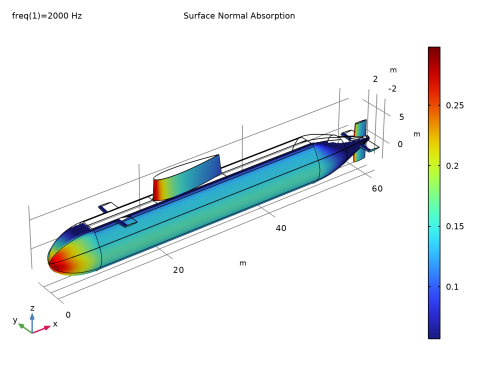
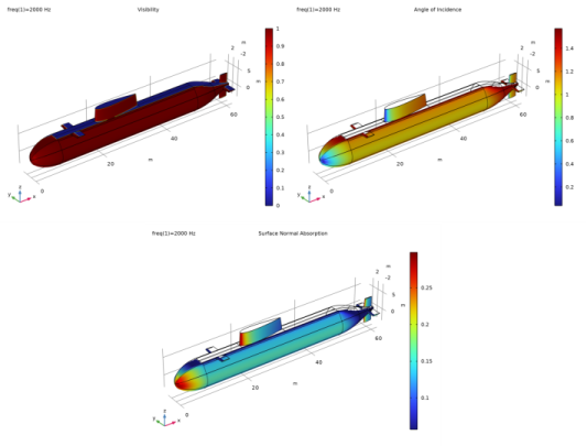
The walls (visible) of the scattering object can be characterized in terms of a reflection coefficient R (complex valued), a normal impedance Zn (complex valued), or an absorption coefficient α and phase. The reflection coefficient and the absorption coefficient can have a dependency on the angle of incidence using the built-in variable paas.theta. If multiple sources are defined, the variable will automatically take the differences into account. Variables also exist for the source defined by the individual background pressure field features, for example, for the first feature paas.bpf1.theta (using the item scope).
|
|
1
|
|
2
|
In the Select Physics tree, select Acoustics > Pressure Acoustics > Pressure Acoustics, Asymptotic Scattering (paas).
|
|
3
|
Click Add.
|
|
4
|
Click
|
|
5
|
|
6
|
Click
|
|
1
|
|
2
|
|
3
|
Click
|
|
4
|
Browse to the model’s Application Libraries folder and double-click the file submarine_asymptotic_scattering_parameters.txt.
|
|
1
|
|
2
|
|
3
|
|
4
|
Click
|
|
5
|
Browse to the model’s Application Libraries folder and double-click the file submarine_asymptotic_scattering_alpha.txt.
|
|
6
|
Click
|
|
7
|
|
8
|
Locate the Interpolation and Extrapolation section. From the Interpolation list, choose Cubic spline.
|
|
9
|
|
10
|
In the Argument table, enter the following settings:
|
|
1
|
|
2
|
|
3
|
Click
|
|
4
|
Browse to the model’s Application Libraries folder and double-click the file submarine_asymptotic_scattering.mphbin.
|
|
5
|
Click
|
|
1
|
|
2
|
On the object fin, select Boundaries 1–10, 69–73, and 79–83 only.
|
|
3
|
|
1
|
|
2
|
On the object cmf1, select Boundaries 4–7, 13–16, 24–27, 49, 50, 62, 63, 65, 66, and 84–87 only.
|
|
3
|
|
4
|
|
5
|
|
6
|
Clear the Automatic detection of small details checkbox.
|
|
7
|
|
1
|
|
2
|
|
3
|
|
4
|
Click
|
|
5
|
Browse to the model’s Application Libraries folder and double-click the file submarine_asymptotic_scattering_variables.txt.
|
|
1
|
|
2
|
|
3
|
|
4
|
|
1
|
|
2
|
Go to the Add Material window.
|
|
3
|
|
4
|
Click the Add to Component button in the window toolbar.
|
|
5
|
|
1
|
|
2
|
|
1
|
In the Model Builder window, under Component 1 (comp1) click Pressure Acoustics, Asymptotic Scattering (paas).
|
|
2
|
In the Settings window for Pressure Acoustics, Asymptotic Scattering, locate the Sound Pressure Level Settings section.
|
|
3
|
From the Reference pressure for the sound pressure level list, choose Use reference pressure for water.
|
|
1
|
In the Model Builder window, under Component 1 (comp1) > Pressure Acoustics, Asymptotic Scattering (paas) click Pressure Acoustics 1.
|
|
2
|
|
3
|
|
1
|
|
2
|
|
3
|
|
4
|
|
5
|
|
1
|
|
2
|
|
3
|
|
4
|
|
1
|
|
1
|
|
2
|
|
3
|
|
1
|
|
2
|
|
3
|
Click the Custom button.
|
|
4
|
Locate the Element Size Parameters section.
|
|
5
|
|
1
|
|
2
|
|
3
|
Click the Custom button.
|
|
4
|
|
5
|
|
1
|
|
3
|
|
1
|
|
2
|
|
3
|
|
4
|
Click
|
|
1
|
|
2
|
|
3
|
|
5
|
|
6
|
Click
|
|
7
|
|
1
|
|
2
|
|
3
|
|
4
|
|
1
|
|
2
|
|
3
|
|
4
|
Click OK.
|
|
5
|
|
6
|
|
7
|
Select the Only plot when requested checkbox.
|
|
8
|
|
1
|
|
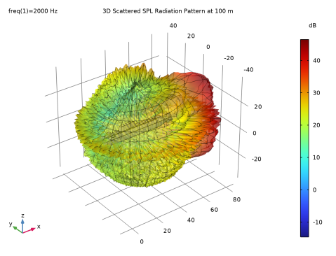
2
|
In the Settings window for 3D Plot Group, type 3D Scattered SPL Radiation Pattern at 100 m in the Label text field.
|
|
3
|
|
1
|
In the Model Builder window, expand the 3D Scattered SPL Radiation Pattern at 100 m node, then click Radiation Pattern 1.
|
|
2
|
|
3
|
|
4
|
|
5
|
|
6
|
|
7
|
|
8
|
|
1
|
In the Model Builder window, right-click 3D Scattered SPL Radiation Pattern at 100 m and choose Surface.
|
|
2
|
|
3
|
|
4
|
|
5
|
|
1
|
|
2
|
|
3
|
|
4
|
|
5
|
|
6
|
|
7
|
|
8
|
|
1
|
|
2
|
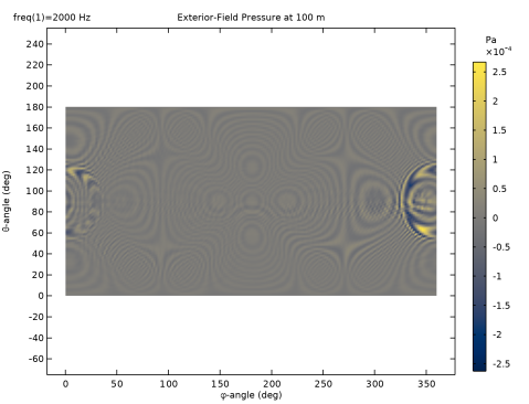
In the Settings window for 2D Plot Group, type Exterior-Field Pressure at 100 m in the Label text field.
|
|
3
|
|
1
|
In the Model Builder window, expand the Exterior-Field Pressure at 100 m node, then click Radiation Pattern 1.
|
|
2
|
|
3
|
|
4
|
|
5
|
|
6
|
|
7
|
|
8
|
|
9
|
|
1
|
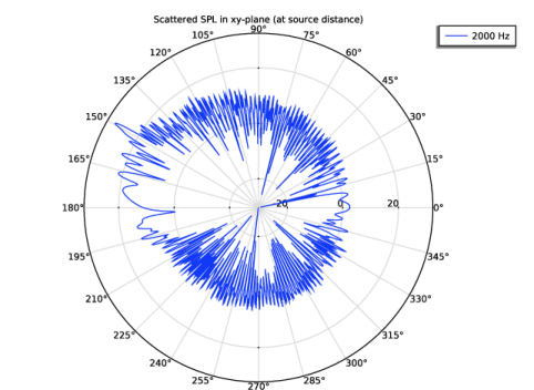
In the Model Builder window, under Results click Exterior-Field Sound Pressure Level xy-plane (paas).
|
|
2
|
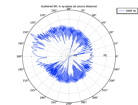
In the Settings window for Polar Plot Group, type Scattered SPL in xy-plane (at source distance) in the Label text field.
|
|
3
|
|
1
|
In the Model Builder window, expand the Scattered SPL in xy-plane (at source distance) node, then click Radiation Pattern 1.
|
|
2
|
|
3
|
|
4
|
|
5
|
|
6
|
|
7
|
Click Preview Evaluation Plane.
|
|
8
|
|
1
|
|
2
|
|
1
|
|
2
|
|
3
|
|
4
|
|
5
|
|
6
|
|
7
|
|
8
|
|
9
|
|
10
|
|
11
|
|
1
|
|
2
|
|
3
|
|
4
|
|
5
|
|
1
|
|
2
|
|
3
|
|
1
|
|
2
|
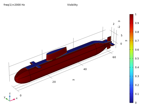
In the Settings window for Surface, click Replace Expression in the upper-right corner of the Expression section. From the menu, choose Component 1 (comp1) > Pressure Acoustics, Asymptotic Scattering > Background Pressure Field 1 > paas.bpf1.visibility - Visibility - 1.
|
|
3
|
|
1
|
|
2
|
|
3
|
|
1
|
|
2
|
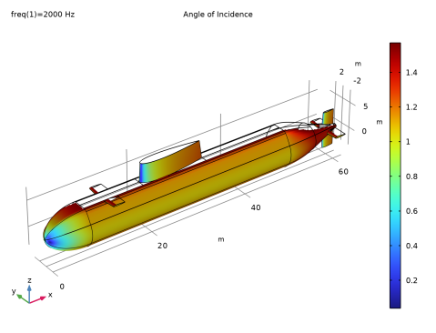
In the Settings window for Surface, click Replace Expression in the upper-right corner of the Expression section. From the menu, choose Component 1 (comp1) > Pressure Acoustics, Asymptotic Scattering > Background Pressure Field 1 > paas.bpf1.theta - Incident angle - rad.
|
|
3
|
Locate the Expression section. In the Expression text field, type if(paas.bpf1.visibility,paas.bpf1.theta,NaN).
|
|
4
|
|
1
|
|
2
|
|
3
|
|
1
|
|
2
|
|
3
|
|
4
|
|
1
|
|
2
|
|
3
|
|
4
|
|
5
|
|
6
|
Select the Only evaluate globally defined expressions checkbox.
|
|
1
|
|
2
|
|
3
|
|
4
|
|
1
|
|
2
|
|
3
|
|
4
|
|
1
|
|
2
|
|
3
|
|
4
|
|
5
|
|
6
|
|
7
|
|
1
|
|
2
|
|
3
|
|
4
|
|
5
|
|
1
|
|
2
|
|
3
|
|
1
|
|
2
|
|
3
|
|
4
|
|
1
|
|
2
|
|
3
|
|
4
|
|
1
|
|
2
|
|
3
|
|
4
|
|
5
|
|
6
|
|
1
|
|
2
|
|
3
|
|
4
|
|
5
|
|
6
|
|
7
|
|
8
|
Select the Scale factor checkbox.
|
|
1
|
|
3
|