PDF

Spherical Scatterer: BEM Benchmark
Introduction
This tutorial models the scattering of a plane wave off a sphere. It is a classic benchmark model for the boundary element method (BEM). When the sphere is modeled as sound hard, the problem has an analytical solution, as described in Ref. 1 and Ref. 2. The model compares the results using the Pressure Acoustics, Boundary Elements interface with the analytical solution for several frequencies. The results show very good agreement. The model results do not show any irregular modes; these can appear as numerical resonances for the inside of the sphere and are sometimes seen when using the BEM method.
Model Definition
The spherical scatterer of radius of 1 m, is depicted in Figure 1. The scatterer is surrounded by an infinite domain of air, with a speed of sound of 343 m/s and a density of 1.225 kg/m3.
Figure 1: Figure 1Spherical scatterer geometry.
The domain is subjected to an incident plane wave traveling in the global x direction. The Background Pressure Field feature is used to set up the incident plane wave and solve this problem. In this situation, the problem is automatically reduced to only solve for the scattered pressure field ps. The total field pt is the sum of the scattered field and the (known) background pressure field pb:
(1)
The plane-wave option defines a background pressure field of the type
(2)
where p0 is the wave amplitude, k is the wave vector with amplitude ks = ω/c and wave direction vector ek, and x is the location on the sphere boundary. The analytical solution for the scattered field ps created by a spherical scatterer under a plane wave in an infinite acoustic domain is given by
(3)
Here, k is the wave number, R is the sphere radius, r = |x − x0| is the distance from the sphere center x0, and N should tend to infinity (we will include 100 terms in the sum). The angle θ is defined such that the shadow zone is located at θ = 0. These expressions are defined in the Variables node in the model.
The expression uses the spherical Bessel functions jn and hn and their derivatives j'n and h'n, which are defined as analytical functions in the model. The Legendre polynomial Pn is a built-in function in COMSOL defined through the expression legendre(l,x).
Results and Discussion
The sound pressure level at 1000 Hz is shown in Figure 2. The BEM solves only on the boundary, but the field obtained through the BEM can be evaluated in any point in the domain that it represents. The figure shows the scattered acoustic sound pressure level on the BEM boundary and its evaluation in the space surrounding the sphere.
Figure 2: Sound pressure level on the BEM boundary and in the spatial domain.
Figure 3 plots the computed exterior-field pressure at a radial distance of 10 m and a frequency of 200 Hz versus azimuthal angle in the positive xy-plane and compares it to the analytical solution. As the plot shows, the computed solution is very close to the analytical solution.
Figure 3: Scattered pressure at f = 200 Hz.
As described in Ref. 3, BEM can present nonuniqueness problems around certain frequencies. The absolute total pressure |pt| is depicted at the point x = (2R000) in Figure 4. From this plot, it is evident that the BEM formulation used does not show any irregular modes, and the solution is in agreement with the analytical solution. Irregular modes would show up as peaks in the solution corresponding to the eigenmodes (resonances) of the interior domain of the sphere.
Figure 4: Absolute total pressure evaluated at x = 2R0.
Notes about the COMSOL implementation
The model and the analytical results may disagree at high frequency if you plot the solution along one of the perimeters of the sphere. This is due to the implementation of the BEM quadrature settings in COMSOL, which are a compromise between performance and accuracy.
If you do want to increase the accuracy of the BEM solution beyond the default settings, you can manually tighten the quadrature settings for BEM feature. To do that, click on Show More Options to activate the Advanced Physics Options to access the quadrature options under the Pressure Acoustics, Boundary Elements physics. Set the Integration orders to manual and change the Integration order of the distant elements, close elements, elements with common vertex, elements with common edge and same element pairs to 4, 6, 6, 6, 6, respectively. Additionally, tighten the tolerance for the solver from the default of 0.01 to 1e-4. You can get a much better agreement with the analytical solution using these changes of the quadrature settings. However, the computational time and memory requirements will increase for the computation.
References
1. M. Hornikx, M. Kaltenbacher, and S. Marburg, “A Platform for Benchmark Cases in Computational Acoustics,” ACTA ACUSTICA UNITED WITH ACUSTICA, vol. 101, pp. 811–820, 2015.
2. S. Marburg, “The Burton and Miller Method: Unlocking Another Mystery if Its Coupling Parameter,” J. Comp. Acoust., vol. 24, p.  15550016, 2016.
3. S. Marburg, “Boundary Element Method for time-harmonic acoustic problems,” Computational Acoustics, CISM International Centre for Mechanical Sciences Courses and Lectures, M. Kaltenbacher, ed., vol. 579, pp.  69–158, 2018.
Application Library path: Acoustics_Module/Verification_Examples/spherical_scatterer_bem_benchmark
Modeling Instructions
From the File menu, choose New.
New
In the New window, click  Model Wizard.
Model Wizard
1
In the Model Wizard window, click  3D.
2
In the Select Physics tree, select Acoustics > Pressure Acoustics > Pressure Acoustics, Boundary Elements (pabe).
3
Click Add.
4
Click  Study.
5
In the Select Study tree, select General Studies > Frequency Domain.
6
Global Definitions
Parameters 1
1
In the Model Builder window, under Global Definitions click Parameters 1.
2
In the Settings window for Parameters, locate the Parameters section.
3
Click  Load from File.
4
Variables - Analytical
1
In the Model Builder window, right-click Global Definitions and choose Variables.
2
In the Settings window for Variables, type Variables - Analytical in the Label text field.
3
Locate the Variables section. Click  Load from File.
4
Analytic 1 (an1)
1
In the Home toolbar, click  Functions and choose Global > Analytic.
2
In the Settings window for Analytic, type J in the Function name text field.
3
Locate the Definition section. In the Expression text field, type sqrt(pi/(2*x))*besselj(n+0.5,x).
4
In the Arguments text field, type n, x.
5
Locate the Units section. In the table, enter the following settings:
6
In the Function text field, type 1.
J is the first type of spherical Bessel functions that will be used in the analytical solution.
Analytic 2 (an2)
1
In the Home toolbar, click  Functions and choose Global > Analytic.
2
In the Settings window for Analytic, type N in the Function name text field.
3
Locate the Definition section. In the Expression text field, type sqrt(pi/(2*x))*bessely(n+0.5,x).
4
In the Arguments text field, type n, x.
5
Locate the Units section. In the table, enter the following settings:
6
In the Function text field, type 1.
N is the second type of spherical Bessel functions that will be used in the analytical solution.
Geometry 1
Sphere 1 (sph1)
1
In the Geometry toolbar, click  Sphere.
2
In the Settings window for Sphere, locate the Size section.
3
In the Radius text field, type R0.
4
Locate the Object Type section. From the Type list, choose Surface.
5
Click  Build All Objects.
The reason for switching the sphere from solid to surface is that the BEM only solves for the unknowns on the boundary, so there is no need to use a volume mesh. The image should look like that in Figure 1.
Mesh 1
Free Triangular 1
1
In the Mesh toolbar, click  More Generators and choose Free Triangular.
2
In the Settings window for Free Triangular, locate the Boundary Selection section.
3
From the Selection list, choose All boundaries.
Size
1
In the Model Builder window, click Size.
2
In the Settings window for Size, locate the Element Size section.
3
Click the Custom button.
4
Locate the Element Size Parameters section. In the Maximum element size text field, type min(0.3,lam0/4).
5
In the Minimum element size text field, type min(0.3,lam0/4).
6
In the Curvature factor text field, type 0.5.
7
In the Resolution of narrow regions text field, type 2.
8
Click  Build All.
The figure shows the mesh which only contains surface elements due to the use of BEM.
Pressure Acoustics, Boundary Elements (pabe)
1
In the Model Builder window, under Component 1 (comp1) click Pressure Acoustics, Boundary Elements (pabe).
2
In the Settings window for Pressure Acoustics, Boundary Elements, locate the Domain Selection section.
3
In the list box, select Finite void 1.
4
Click  Remove from Selection.
5
Pressure Acoustics 1
1
In the Model Builder window, under Component 1 (comp1) > Pressure Acoustics, Boundary Elements (pabe) click Pressure Acoustics 1.
2
In the Settings window for Pressure Acoustics, locate the Pressure Acoustics Model section.
3
From the c list, choose User defined. In the associated text field, type c0.
4
From the ρ list, choose User defined. In the associated text field, type rho0.
Background Pressure Field 1
1
In the Physics toolbar, click  Domains and choose Background Pressure Field.
2
In the Settings window for Background Pressure Field, locate the Background Pressure Field section.
3
In the p0 text field, type 1.
Study 1
Step 1: Frequency Domain
1
In the Model Builder window, under Study 1 click Step 1: Frequency Domain.
2
In the Settings window for Frequency Domain, locate the Study Settings section.
3
In the Frequencies text field, type range(50,50,f0).
4
In the Model Builder window, click Study 1.
5
In the Settings window for Study, locate the Study Settings section.
6
Clear the Generate default plots checkbox.
7
In the Study toolbar, click  Compute.
Results
In the Model Builder window, expand the Results node.
Grid 3D 1
1
In the Model Builder window, expand the Results > Datasets node.
2
Right-click Results > Datasets and choose More 3D Datasets > Grid 3D.
3
In the Settings window for Grid 3D, locate the Parameter Bounds section.
4
Find the First parameter subsection. In the Minimum text field, type -3.
5
In the Maximum text field, type 5.
6
Find the Second parameter subsection. In the Minimum text field, type -3.
7
In the Maximum text field, type 3.
8
Find the Third parameter subsection. In the Minimum text field, type -3.
9
In the Maximum text field, type 3.
10
Click to expand the Grid section. In the x resolution text field, type 100.
11
In the y resolution text field, type 40.
12
In the z resolution text field, type 100.
Parametric Curve 3D 1
1
In the Results toolbar, click  More Datasets and choose Parametric Curve 3D.
2
In the Settings window for Parametric Curve 3D, locate the Expressions section.
3
In the x text field, type R0+5*R0*s.
4
Select the Only evaluate globally defined expressions checkbox.
Cut Point 3D 1
1
In the Results toolbar, click  Cut Point 3D.
2
In the Settings window for Cut Point 3D, locate the Data section.
3
From the Dataset list, choose Grid 3D 1.
4
Locate the Point Data section. In the x text field, type 2*R0.
5
In the y text field, type 0.
6
In the z text field, type 0.
Acoustic Pressure, Boundaries (pabe)
1
In the Results toolbar, click  3D Plot Group.
2
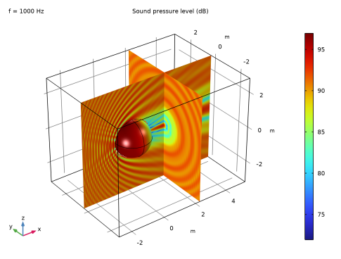
In the Settings window for 3D Plot Group, type Acoustic Pressure, Boundaries (pabe) in the Label text field.
3
Locate the Data section. From the Parameter value (freq (Hz)) list, choose 1000.
4
Click to expand the Title section. From the Title type list, choose Manual.
5
In the Title text area, type Total acoustic pressure (Pa).
6
In the Parameter indicator text field, type f = eval(freq) Hz.
Surface 1
1
Right-click Acoustic Pressure, Boundaries (pabe) and choose Surface.
2
In the Settings window for Surface, locate the Expression section.
3
In the Expression text field, type pabe.p_t_bnd.
4
Locate the Coloring and Style section. From the Scale list, choose Linear symmetric.
5
From the Color table list, choose Wave.
6
In the Acoustic Pressure, Boundaries (pabe) toolbar, click  Plot.
The image shows the total acoustic pressure on the boundary.
Acoustic Pressure (pabe)
1
In the Results toolbar, click  3D Plot Group.
2
In the Settings window for 3D Plot Group, type Acoustic Pressure (pabe) in the Label text field.
3
Locate the Data section. From the Parameter value (freq (Hz)) list, choose 500.
4
Locate the Title section. From the Title type list, choose Manual.
5
In the Parameter indicator text field, type f = eval(freq) Hz.
6
In the Title text area, type Total acoustic pressure field (Pa).
Multislice 1
1
In the Acoustic Pressure (pabe) toolbar, click  More Plots and choose Multislice.
2
In the Settings window for Multislice, locate the Multiplane Data section.
3
Find the X-planes subsection. In the Planes text field, type 0.
4
Locate the Coloring and Style section. From the Scale list, choose Linear symmetric.
5
From the Color table list, choose Wave.
Line 1
1
In the Model Builder window, right-click Acoustic Pressure (pabe) and choose Line.
2
In the Settings window for Line, locate the Expression section.
3
In the Expression text field, type 1.
4
Locate the Coloring and Style section. From the Coloring list, choose Uniform.
5
From the Color list, choose Black.
Acoustic Pressure (pabe)
1
In the Model Builder window, click Acoustic Pressure (pabe).
2
In the Settings window for 3D Plot Group, locate the Data section.
3
From the Dataset list, choose Grid 3D 1.
Line 1
1
In the Model Builder window, click Line 1.
2
In the Settings window for Line, locate the Data section.
3
From the Dataset list, choose Study 1/Solution 1 (sol1).
4
From the Solution parameters list, choose From parent.
5
Click to expand the Title section. From the Title type list, choose None.
Surface 1
1
In the Model Builder window, right-click Acoustic Pressure (pabe) and choose Surface.
2
In the Settings window for Surface, locate the Expression section.
3
In the Expression text field, type pabe.p_t_bnd.
4
Click to expand the Inherit Style section. From the Plot list, choose Multislice 1.
5
Locate the Data section. From the Dataset list, choose Study 1/Solution 1 (sol1).
6
From the Solution parameters list, choose From parent.
7
In the Acoustic Pressure (pabe) toolbar, click  Plot.
The image shows the total acoustic pressure on the boundary and its evaluation in the spatial grid.
Sound Pressure Level (pabe)
1
In the Results toolbar, click  3D Plot Group.
2
In the Settings window for 3D Plot Group, type Sound Pressure Level (pabe) in the Label text field.
3
Locate the Data section. From the Dataset list, choose Grid 3D 1.
4
From the Parameter value (freq (Hz)) list, choose 1000.
5
Locate the Title section. From the Title type list, choose Manual.
6
In the Parameter indicator text field, type f = eval(freq) Hz.
7
In the Title text area, type Sound pressure level (dB).
Multislice 1
1
In the Sound Pressure Level (pabe) toolbar, click  More Plots and choose Multislice.
2
In the Settings window for Multislice, locate the Expression section.
3
In the Expression text field, type pabe.Lp_t.
4
Locate the Multiplane Data section. Find the x-planes subsection. From the Entry method list, choose Coordinates.
5
In the Coordinates text field, type 2.
6
Find the z-planes subsection. In the Planes text field, type 0.
Line 1
1
In the Model Builder window, right-click Sound Pressure Level (pabe) and choose Line.
2
In the Settings window for Line, locate the Data section.
3
From the Dataset list, choose Study 1/Solution 1 (sol1).
4
From the Solution parameters list, choose From parent.
5
Locate the Expression section. In the Expression text field, type 1.
6
Locate the Coloring and Style section. From the Coloring list, choose Uniform.
7
From the Color list, choose Black.
8
Locate the Title section. From the Title type list, choose None.
Surface 1
1
Right-click Sound Pressure Level (pabe) and choose Surface.
2
In the Settings window for Surface, locate the Expression section.
3
In the Expression text field, type pabe.Lp_t_bnd.
4
Locate the Inherit Style section. From the Plot list, choose Multislice 1.
5
Locate the Data section. From the Dataset list, choose Study 1/Solution 1 (sol1).
6
From the Solution parameters list, choose From parent.
7
In the Sound Pressure Level (pabe) toolbar, click  Plot.
The image should look like that in Figure 2.
Scattered Pressure in the xy-plane
1
In the Results toolbar, click  Polar Plot Group.
2
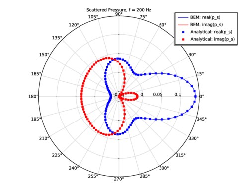
In the Settings window for Polar Plot Group, type Scattered Pressure in the xy-plane in the Label text field.
3
Locate the Data section. From the Parameter selection (freq) list, choose From list.
4
In the Parameter values (freq (Hz)) list box, select 200.
5
Click to expand the Title section. From the Title type list, choose Manual.
6
From the Number format list, choose Automatic.
7
In the Precision text field, type 4.
8
In the Title text area, type Scattered Pressure, f = eval(freq) Hz.
Radiation Pattern 1
1
In the Scattered Pressure in the xy-plane toolbar, click  More Plots and choose Radiation Pattern.
2
In the Settings window for Radiation Pattern, locate the Expression section.
3
In the Expression text field, type real(pabe.p_s).
4
Locate the Evaluation section. Find the Angles subsection. In the Number of angles text field, type 360.
5
Find the Evaluation distance subsection. In the Radius text field, type 10.
6
Click to expand the Legends section. Select the Show legends checkbox.
7
From the Legends list, choose Manual.
8
9
Click to expand the Coloring and Style section. From the Color list, choose Blue.
Scattered Pressure in the xy-plane
In the Model Builder window, click Scattered Pressure in the xy-plane.
Radiation Pattern 2
1
In the Scattered Pressure in the xy-plane toolbar, click  More Plots and choose Radiation Pattern.
2
In the Settings window for Radiation Pattern, locate the Expression section.
3
In the Expression text field, type imag(pabe.p_s).
4
Locate the Evaluation section. Find the Angles subsection. In the Number of angles text field, type 360.
5
Find the Evaluation distance subsection. In the Radius text field, type 10.
6
Locate the Legends section. Select the Show legends checkbox.
7
From the Legends list, choose Manual.
8
9
Locate the Coloring and Style section. From the Color list, choose Red.
Scattered Pressure in the xy-plane
In the Model Builder window, click Scattered Pressure in the xy-plane.
Radiation Pattern 3
1
In the Scattered Pressure in the xy-plane toolbar, click  More Plots and choose Radiation Pattern.
2
In the Settings window for Radiation Pattern, locate the Expression section.
3
In the Expression text field, type real(pana).
4
Locate the Evaluation section. Find the Angles subsection. In the Number of angles text field, type 90.
5
Find the Evaluation distance subsection. In the Radius text field, type 10.
6
Locate the Legends section. Select the Show legends checkbox.
7
From the Legends list, choose Manual.
8
9
Locate the Coloring and Style section. Find the Line style subsection. From the Line list, choose None.
10
From the Color list, choose Blue.
11
Find the Line markers subsection. From the Marker list, choose Point.
Scattered Pressure in the xy-plane
In the Model Builder window, click Scattered Pressure in the xy-plane.
Radiation Pattern 4
1
In the Scattered Pressure in the xy-plane toolbar, click  More Plots and choose Radiation Pattern.
2
In the Settings window for Radiation Pattern, locate the Expression section.
3
In the Expression text field, type imag(pana).
4
Locate the Evaluation section. Find the Angles subsection. In the Number of angles text field, type 90.
5
Find the Evaluation distance subsection. In the Radius text field, type 10.
6
Locate the Legends section. Select the Show legends checkbox.
7
From the Legends list, choose Manual.
8
9
Locate the Coloring and Style section. Find the Line style subsection. From the Line list, choose None.
10
From the Color list, choose Red.
11
Find the Line markers subsection. From the Marker list, choose Point.
12
From the Positioning list, choose In evaluation points.
13
In the Scattered Pressure in the xy-plane toolbar, click  Plot.
The image should look like that in Figure 3.
Scattered SPL in the xy-plane
1
In the Results toolbar, click  Polar Plot Group.
2
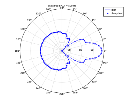
In the Settings window for Polar Plot Group, type Scattered SPL in the xy-plane in the Label text field.
3
Locate the Data section. From the Parameter selection (freq) list, choose From list.
4
In the Parameter values (freq (Hz)) list box, select 500.
5
Locate the Title section. From the Title type list, choose Manual.
6
From the Number format list, choose Automatic.
7
In the Precision text field, type 4.
8
In the Title text area, type Scattered SPL, f = eval(freq) Hz.
Radiation Pattern 1
1
In the Scattered SPL in the xy-plane toolbar, click  More Plots and choose Radiation Pattern.
2
In the Settings window for Radiation Pattern, locate the Expression section.
3
In the Expression text field, type pabe.Lp_s.
4
Locate the Evaluation section. Find the Angles subsection. In the Number of angles text field, type 360.
5
Find the Evaluation distance subsection. In the Radius text field, type 2.
6
Locate the Legends section. Select the Show legends checkbox.
7
From the Legends list, choose Manual.
8
9
Locate the Coloring and Style section. From the Color list, choose Blue.
Scattered SPL in the xy-plane
In the Model Builder window, click Scattered SPL in the xy-plane.
Radiation Pattern 2
1
In the Scattered SPL in the xy-plane toolbar, click  More Plots and choose Radiation Pattern.
2
In the Settings window for Radiation Pattern, locate the Expression section.
3
In the Expression text field, type 20*log10(sqrt(0.5)*abs(pana)/pabe.pref_SPL).
4
Locate the Evaluation section. Find the Angles subsection. In the Number of angles text field, type 90.
5
Find the Evaluation distance subsection. In the Radius text field, type 2.
6
Locate the Legends section. Select the Show legends checkbox.
7
From the Legends list, choose Manual.
8
9
Locate the Coloring and Style section. Find the Line style subsection. From the Line list, choose None.
10
From the Color list, choose Blue.
11
Find the Line markers subsection. From the Marker list, choose Point.
12
From the Positioning list, choose In evaluation points.
13
In the Scattered SPL in the xy-plane toolbar, click  Plot.
The image shows the scattered sound pressure level in the xy-plane and its comparison with the analytical solution.
Scattered Pressure along the x-axis
1
In the Results toolbar, click  1D Plot Group.
2
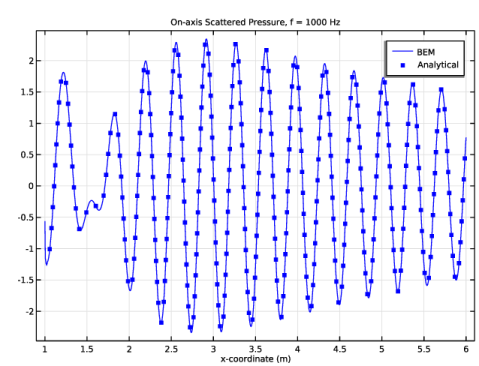
In the Settings window for 1D Plot Group, type Scattered Pressure along the x-axis in the Label text field.
3
Locate the Data section. From the Dataset list, choose Parametric Curve 3D 1.
4
From the Parameter selection (freq) list, choose From list.
5
In the Parameter values (freq (Hz)) list box, select 1000.
6
Click to expand the Title section. From the Title type list, choose Manual.
7
From the Number format list, choose Automatic.
8
In the Precision text field, type 4.
9
In the Title text area, type On-axis Scattered Pressure, f = eval(freq) Hz.
Line Graph 1
1
Right-click Scattered Pressure along the x-axis and choose Line Graph.
2
In the Settings window for Line Graph, locate the y-Axis Data section.
3
In the Expression text field, type pabe.p_s.
4
Locate the x-Axis Data section. From the Parameter list, choose Expression.
5
In the Expression text field, type x.
6
Click to expand the Coloring and Style section. From the Color list, choose Blue.
7
Click to expand the Legends section. Select the Show legends checkbox.
8
From the Legends list, choose Manual.
9
Line Graph 2
1
In the Model Builder window, right-click Scattered Pressure along the x-axis and choose Line Graph.
2
In the Settings window for Line Graph, locate the y-Axis Data section.
3
In the Expression text field, type pana.
4
Locate the x-Axis Data section. From the Parameter list, choose Expression.
5
In the Expression text field, type x.
6
Locate the Coloring and Style section. From the Color list, choose Blue.
7
Find the Line style subsection. From the Line list, choose None.
8
Find the Line markers subsection. From the Marker list, choose Point.
9
From the Positioning list, choose Interpolated.
10
In the Number text field, type 300.
11
Locate the Legends section. Select the Show legends checkbox.
12
From the Legends list, choose Manual.
13
14
In the Scattered Pressure along the x-axis toolbar, click  Plot.
The image shows the scattered pressure along the x-axis and its comparison with the analytical solution.
Absolute Total Pressure in Point
1
In the Results toolbar, click  1D Plot Group.
2
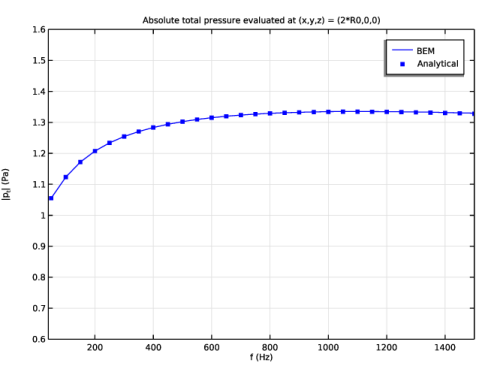
In the Settings window for 1D Plot Group, type Absolute Total Pressure in Point in the Label text field.
3
Locate the Data section. From the Dataset list, choose Cut Point 3D 1.
4
Locate the Title section. From the Title type list, choose Manual.
5
In the Title text area, type Absolute total pressure evaluated at (x,y,z) = (2*R0,0,0).
6
Locate the Plot Settings section.
7
Select the x-axis label checkbox. In the associated text field, type f (Hz).
8
Select the y-axis label checkbox. In the associated text field, type |p<sub>t</sub>| (Pa).
9
Locate the Axis section. Select the Manual axis limits checkbox.
10
In the x minimum text field, type 40.
11
In the x maximum text field, type 1500.
12
In the y minimum text field, type 0.6.
13
In the y maximum text field, type 1.6.
Point Graph 1
1
Right-click Absolute Total Pressure in Point and choose Point Graph.
2
In the Settings window for Point Graph, locate the y-Axis Data section.
3
In the Expression text field, type abs(pabe.p_t).
4
Click to expand the Legends section. Select the Show legends checkbox.
5
From the Legends list, choose Manual.
6
7
Click to expand the Title section. Click to expand the Coloring and Style section. From the Color list, choose Blue.
Point Graph 2
1
In the Model Builder window, right-click Absolute Total Pressure in Point and choose Point Graph.
2
In the Settings window for Point Graph, locate the y-Axis Data section.
3
In the Expression text field, type abs(pana+pabe.p_b).
4
Locate the Legends section. Select the Show legends checkbox.
5
From the Legends list, choose Manual.
6
7
Locate the Coloring and Style section. Find the Line style subsection. From the Line list, choose None.
8
From the Color list, choose Blue.
9
Find the Line markers subsection. From the Marker list, choose Point.
10
In the Absolute Total Pressure in Point toolbar, click  Plot.
The image should look like that in Figure 4.