PDF

Sound Radiation from a Circular Duct with Flow
Introduction
Model of the sound radiation from a circular duct with uniform flow. The convected acoustic problem is described using the linearized potential flow equations solved in the frequency domain. The acoustic inlet is treated including higher order modes using the Port boundary condition.
Model Definition
The mode consists of a duct of radius a placed in a uniform axial flow with magnitude U0. The duct is open at one end radiating sound into an infinite domain; see Figure 1. The setup mimics a very simplified and conceptual engine intake configuration. The single-mode radiation from the duct and the spatial radiation characteristics are computed. The modal content and the nonreflecting condition at the duct inlet are set up using Port boundary conditions. One mode is excited (incident) while all propagating outgoing modes are included at the port boundary. The model parameters and model setup is inspired by Ref. 1.
Figure 1: Sketch of the problem setup, showing a duct open at one end and excited at the port.
The model reproduces the pressure radiation pattern from Figure 8 (b) in Ref. 1, by using the duct radius 0.085 m, Mach number 0.12, and flow velocity parameters from Table 1 in Ref. 1. The excited mode is the (m,n) = (1,0) mode.
Results and Discussion
The radiation pattern evaluated at 2 m from the duct entrance is depicted in Figure 2. Note that the SPL value evaluated in COMSOL is corrected to represent the peak value to match the result from Ref. 1. The pressure field in the (r,z)-plane (0 azimuthal angle) is depicted in Figure 3. The pressure field including the azimuthal component is depicted in Figure 4 and Figure 5. The sound pressure level (RMS based) is depicted in Figure 6 and Figure 7.
Figure 2: Radiation pattern evaluated at 2 m.
Figure 3: Acoustic pressure in the (r,z)-plane (0 azimuthal angle).
Figure 4: Acoustic pressure represented in 3D including the azimuthal component.
Figure 5: Acoustic pressure represented in two z-cut planes including the azimuthal component of the acoustic field.
Figure 6: The sound pressure level evaluated in the (r,z)-plane.
Figure 7: The sound pressure level evaluated in 3D.
Reference
1. C. Ford, A. Pereira, and C. Bailly, “Radiation of higher order modes from circular ducts with flow,” Acta Acustica, vol. 7, 2023.
Article available at: acta-acustica.edpsciences.org/articles/aacus/full_html/2023/01/aacus220052/aacus220052.html. Copyright The Author(s), published by EDP Sciences, 2023. This Article is published under the Creative Commons Attribution 4.0 International license: creativecommons.org/licenses/by/4.0/. The model Sound Radiation from a Circular Duct with Flow reproduces the pressure radiation pattern from Figure 8 (b), by using the duct radius, Mach number, and flow velocity parameters from Table 1.
Application Library path: Acoustics_Module/Aeroacoustics_and_Noise/sound_radiation_circular_duct
Modeling Instructions
From the File menu, choose New.
New
In the New window, click  Model Wizard.
Model Wizard
1
In the Model Wizard window, click  2D Axisymmetric.
2
In the Select Physics tree, select Acoustics > Aeroacoustics > Linearized Potential Flow, Frequency Domain (lpff).
3
Click Add.
4
Click  Study.
5
In the Select Study tree, select General Studies > Frequency Domain.
6
Global Definitions
Parameters 1
1
In the Model Builder window, under Global Definitions click Parameters 1.
2
In the Settings window for Parameters, locate the Parameters section.
3
Click  Load from File.
4
Geometry 1
Circle 1 (c1)
1
In the Model Builder window, expand the Component 1 (comp1) > Geometry 1 node.
2
Right-click Geometry 1 and choose Circle.
3
In the Settings window for Circle, locate the Size and Shape section.
4
In the Radius text field, type 1.4*R0.
5
In the Sector angle text field, type 180.
6
Locate the Rotation Angle section. In the Rotation text field, type -90.
7
Click to expand the Layers section. In the table, enter the following settings:
Rectangle 1 (r1)
1
In the Geometry toolbar, click  Rectangle.
2
In the Settings window for Rectangle, locate the Size and Shape section.
3
In the Width text field, type a.
4
In the Height text field, type 1.5*R0.
5
Locate the Position section. In the z text field, type -1.5*R0.
6
Click to expand the Layers section. In the table, enter the following settings:
7
Clear the Layers on bottom checkbox.
8
Select the Layers on top checkbox.
Union 1 (uni1)
1
In the Geometry toolbar, click  Booleans and Partitions and choose Union.
2
Click in the Graphics window and then press Ctrl+A to select both objects.
Delete Entities 1 (del1)
1
Right-click Geometry 1 and choose Delete Entities.
2
In the Settings window for Delete Entities, locate the Entities or Objects to Delete section.
3
From the Geometric entity level list, choose Domain.
4
On the object uni1, select Domains 1–4 only.
Form Union (fin)
In the Geometry toolbar, click  Build All.
Materials
Material 1 (mat1)
1
In the Model Builder window, under Component 1 (comp1) right-click Materials and choose Blank Material.
2
In the Settings window for Material, click to expand the Material Properties section.
3
In the Material properties tree, select Basic Properties > Density.
4
Click  Add to Material.
5
In the Material properties tree, select Basic Properties > Speed of Sound.
6
Click  Add to Material.
7
Locate the Material Contents section. In the table, enter the following settings:
Mesh 1
In this model, the mesh is set up manually. Proceed by directly adding the desired mesh component. The mesh includes boundary layers which are there to control and create a fine mesh near the edge of the pipe. The well resolved pipe corner as well as a good resolution of the wavelength in the model is necessary to get an accurate radiation pattern.
Mapped 1
1
In the Mesh toolbar, click  Mapped.
2
In the Settings window for Mapped, locate the Domain Selection section.
3
From the Geometric entity level list, choose Domain.
4
Distribution 1
1
Right-click Mapped 1 and choose Distribution.
2
3
In the Settings window for Distribution, locate the Distribution section.
4
In the Number of elements text field, type 12.
Size
1
In the Model Builder window, under Component 1 (comp1) > Mesh 1 click Size.
2
In the Settings window for Size, locate the Element Size section.
3
Click the Custom button.
In general, 5 to 6 second-order elements per wavelength are needed to resolve the waves. For more details, see Meshing (Resolving the Waves) in the Acoustics Module User’s Guide .
4
Locate the Element Size Parameters section. In the Maximum element size text field, type (c0-U0)/f0/6.
5
In the Minimum element size text field, type (c0-U0)/f0/10.
Boundary Layers 1
1
In the Mesh toolbar, click  Boundary Layers.
2
In the Settings window for Boundary Layers, locate the Domain Selection section.
3
From the Geometric entity level list, choose Domain.
4
5
Click to expand the Transition section. Clear the Smooth transition to interior mesh checkbox.
Boundary Layer Properties
1
In the Model Builder window, click Boundary Layer Properties.
2
3
In the Settings window for Boundary Layer Properties, locate the Layers section.
4
In the Number of layers text field, type 2.
5
In the Thickness adjustment factor text field, type 3.
Boundary Layers 2
1
In the Mesh toolbar, click  Boundary Layers.
2
In the Settings window for Boundary Layers, locate the Domain Selection section.
3
From the Geometric entity level list, choose Domain.
4
5
Locate the Transition section. Clear the Smooth transition to interior mesh checkbox.
Boundary Layer Properties
1
In the Model Builder window, click Boundary Layer Properties.
2
3
In the Settings window for Boundary Layer Properties, locate the Layers section.
4
In the Number of layers text field, type 2.
5
In the Thickness adjustment factor text field, type 3.
Free Triangular 1
1
In the Mesh toolbar, click  Free Triangular.
2
In the Settings window for Free Triangular, locate the Domain Selection section.
3
From the Geometric entity level list, choose Domain.
4
Size 1
1
Right-click Free Triangular 1 and choose Size.
2
In the Settings window for Size, locate the Element Size section.
3
Click the Custom button.
4
Locate the Element Size Parameters section.
5
Select the Maximum element size checkbox. In the associated text field, type (c0-U0)/f0/6.
Mapped 2
In the Mesh toolbar, click  Mapped.
Distribution 1
1
Right-click Mapped 2 and choose Distribution.
2
3
In the Settings window for Distribution, locate the Distribution section.
4
In the Number of elements text field, type 20.
5
Click  Build All.
Proceed to set up the physics. The Port conditions are used at the source to excite the desired mode (m,n)=(1,0), as well as absorb reflected acoustic modes. The reflected modes are generated due to the impedance jump at the pipe opening. It is necessary to include the radial modes n=1 and n=2 also.
Linearized Potential Flow, Frequency Domain (lpff)
In a 2D axisymmetric model the azimuthal mode number (m) is set at the physics interface level. Also choose the desired mode scaling. The power scaling will ensure that the absolute levels seen in the reference paper are achieved.
1
In the Model Builder window, under Component 1 (comp1) click Linearized Potential Flow, Frequency Domain (lpff).
2
In the Settings window for Linearized Potential Flow, Frequency Domain, locate the Linearized Potential Flow Equation Settings section.
3
In the m text field, type m.
4
Locate the Global Port Settings section. From the Mode shape normalization list, choose Power normalization.
Linearized Potential Flow Model 1
1
In the Model Builder window, under Component 1 (comp1) > Linearized Potential Flow, Frequency Domain (lpff) click Linearized Potential Flow Model 1.
2
In the Settings window for Linearized Potential Flow Model, locate the Model Input section.
3
Specify the u0 vector as
Interior Sound Hard Boundary (Wall) 1
1
In the Physics toolbar, click  Boundaries and choose Interior Sound Hard Boundary (Wall).
2
Port 1
1
In the Physics toolbar, click  Boundaries and choose Port.
2
3
In the Settings window for Port, locate the Port Properties section.
4
From the Type of port list, choose Circular.
5
Locate the Port Incident Mode Settings section. From the Incident wave excitation at this port list, choose On.
6
From the Define incident wave list, choose Mode scale.
7
In the Sin text field, type 1.
Port 2
1
In the Physics toolbar, click  Boundaries and choose Port.
2
3
In the Settings window for Port, locate the Port Properties section.
4
From the Type of port list, choose Circular.
5
Locate the Port Mode Settings section. In the n text field, type 1.
Port 3
1
In the Physics toolbar, click  Boundaries and choose Port.
2
3
In the Settings window for Port, locate the Port Properties section.
4
From the Type of port list, choose Circular.
5
Locate the Port Mode Settings section. In the n text field, type 2.
Definitions
Perfectly Matched Layer 1 (pml1)
1
In the Definitions toolbar, click  Perfectly Matched Layer.
2
3
In the Settings window for Perfectly Matched Layer, locate the Scaling section.
4
In the PML scaling curvature parameter text field, type 3.
Study 1
Step 1: Frequency Domain
1
In the Model Builder window, under Study 1 click Step 1: Frequency Domain.
2
In the Settings window for Frequency Domain, locate the Study Settings section.
3
In the Frequencies text field, type f0.
4
In the Model Builder window, click Study 1.
5
In the Settings window for Study, type Study 1 - Frequency Domain in the Label text field.
6
In the Study toolbar, click  Compute.
Results
Acoustic Pressure (lpff)
Now, look at the default plots and make some modifications, like adding selections to the physical domain (excluding the PML).
1
In the Settings window for 2D Plot Group, click to expand the Selection section.
2
From the Geometric entity level list, choose Domain.
3
4
Select the Apply to dataset edges checkbox.
5
In the Acoustic Pressure (lpff) toolbar, click  Plot.
6
Click the  Zoom Extents button in the Graphics toolbar.
Sound Pressure Level (lpff)
1
In the Model Builder window, click Sound Pressure Level (lpff).
2
In the Settings window for 2D Plot Group, locate the Selection section.
3
From the Geometric entity level list, choose Domain.
4
5
Select the Apply to dataset edges checkbox.
6
In the Sound Pressure Level (lpff) toolbar, click  Plot.
7
Click the  Zoom Extents button in the Graphics toolbar.
Revolution 2D
In the Model Builder window, expand the Results > Datasets node, then click Revolution 2D.
Selection
1
In the Results toolbar, click  Attributes and choose Selection.
2
In the Settings window for Selection, locate the Geometric Entity Selection section.
3
From the Geometric entity level list, choose Domain.
4
Surface
1
In the Model Builder window, expand the Acoustic Pressure, 3D (lpff) node, then click Surface.
2
In the Settings window for Surface, locate the Expression section.
3
In the Expression text field, type lpff.p*exp(i*m*rev1phi).
4
In the Acoustic Pressure, 3D (lpff) toolbar, click  Plot.
5
Click the  Zoom Extents button in the Graphics toolbar.
Sound Pressure Level, 3D (lpff)
1
In the Model Builder window, under Results click Sound Pressure Level, 3D (lpff).
2
In the Sound Pressure Level, 3D (lpff) toolbar, click  Plot.
3
Click the  Zoom Extents button in the Graphics toolbar.
Radiation Pattern
1
In the Results toolbar, click  Polar Plot Group.
2
In the Settings window for Polar Plot Group, type Radiation Pattern in the Label text field.
3
Click to expand the Title section. From the Title type list, choose Label.
4
Locate the Axis section. Select the Manual axis limits checkbox.
5
In the r maximum text field, type 80.
6
Select the Symmetric angle range checkbox.
7
From the Zero angle list, choose Up.
8
From the Rotation direction list, choose Clockwise.
9
Locate the Grid section. Select the Manual spacing checkbox.
10
In the θ spacing text field, type 10.
11
In the r spacing text field, type 16.
Line Graph 1
1
In the Radiation Pattern toolbar, click  Line Graph.
2
Here, the extra term transforms form the RMS level to the peak level, this is the typical 3 dB correction.
3
In the Settings window for Line Graph, locate the r-Axis Data section.
4
In the Expression text field, type lpff.Lp+20*log10(sqrt(2))[dB].
Define the polar angle expression.
5
Locate the θ Angle Data section. From the Parameter list, choose Expression.
6
In the Expression text field, type atan2(z,r).
7
In the Radiation Pattern toolbar, click  Plot.
Now, also create a 3D plot of the pressure just below and above the pipe entrance. For this create a new dataset where the selection is restricted to the outside air domain.
Revolution 2D 2
In the Model Builder window, right-click Revolution 2D and choose Duplicate.
Selection
1
In the Model Builder window, expand the Revolution 2D 2 node, then click Selection.
2
Acoustic Pressure, 3D Slices
1
In the Home toolbar, click  Add Plot Group and choose 3D Plot Group.
2
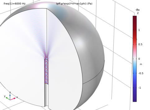
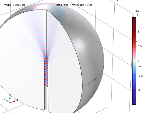
In the Settings window for 3D Plot Group, type Acoustic Pressure, 3D Slices in the Label text field.
3
Locate the Data section. From the Dataset list, choose Revolution 2D 2.
4
Locate the Color Legend section. Select the Show units checkbox.
Slice 1
1
Right-click Acoustic Pressure, 3D Slices and choose Slice.
2
In the Settings window for Slice, locate the Expression section.
3
In the Expression text field, type lpff.p*exp(i*m*rev1phi).
4
Locate the Plane Data section. From the Plane list, choose XY-planes.
5
From the Entry method list, choose Coordinates.
6
In the Z-coordinates text field, type -0.1 0.5.
7
Locate the Coloring and Style section. From the Color table list, choose Wave.
8
From the Scale list, choose Linear symmetric.
9
In the Acoustic Pressure, 3D Slices toolbar, click  Plot.
Finally, add an evaluation group computing the power of the incident and reflected (outgoing) port modes.
Evaluation Group 1 - Port Mode Powers
1
In the Results toolbar, click  Evaluation Group.
2
In the Settings window for Evaluation Group, type Evaluation Group 1 - Port Mode Powers in the Label text field.
Global Evaluation 1
1
Right-click Evaluation Group 1 - Port Mode Powers and choose Global Evaluation.
2
In the Settings window for Global Evaluation, click Replace Expression in the upper-right corner of the Expressions section. From the menu, choose Component 1 (comp1) > Linearized Potential Flow, Frequency Domain > Ports > Port 1 > lpff.port1.P_in - Power of incident mode - W.
3
Locate the Expressions section. In the table, enter the following settings:
4
In the Evaluation Group 1 - Port Mode Powers toolbar, click  Evaluate.