|
|
|
|
d
|
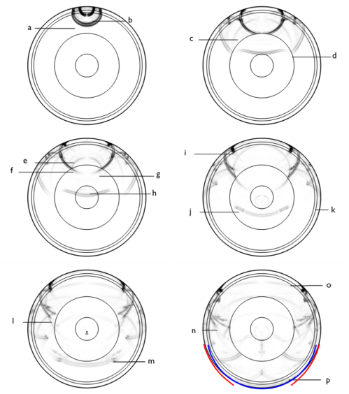
The p-waves reaching the outer core are partially transmitted as p-waves traveling through the liquid. The p-waves that have not been transmitted to the outer core or reflected back continue their travel. This leaves part of Earth without direct p-waves. This is called the p-waves shadow zone and it was quite relevant to identify the internal structure of Earth at the early stages of the development of seismology.
|
|
i
|
The existence of discontinuities in the outer most layers create a series of refracted waves called head waves or von Schmidt waves.
|
|
k
|
|
l
|
The s-waves continue to travel through the mantle without reaching all of Earth. This area where no s-waves are transmitted is called the s-wave shadow zone. As the shear waves cannot travel through fluids, these are the only direct s-waves still existing.
|
|
n
|
The s-waves finally reach the surface of Earth. This point defines the start of the s-waves shadow zone, marked in blue.
|
|
o
|
The Rayleigh waves, which are slower than the s-waves, can be seen a this point.
|
|
p
|
The p-waves that have traveled through the core finally reach the other side of Earth, defining the other end of the p-waves shadow zone, marked in red.
|
|
1
|
|
2
|
In the Select Physics tree, select Acoustics > Pressure Acoustics > Pressure Acoustics, Time Explicit (pate).
|
|
3
|
Click Add.
|
|
4
|
|
5
|
Click Add.
|
|
6
|
Click
|
|
7
|
|
8
|
Click
|
|
1
|
|
2
|
|
3
|
Click
|
|
4
|
Browse to the model’s Application Libraries folder and double-click the file seismic_waves_earth_parameters.txt.
|
|
1
|
|
2
|
|
3
|
|
4
|
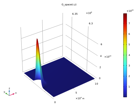
Locate the Definition section. In the Expression text field, type 10e26/sqrt(pi*dS)*exp(-((r - r0)^2 + (z - z0)^2)/dS).
|
|
5
|
|
6
|
Locate the Units section. In the table, enter the following settings:
|
|
7
|
|
8
|
Locate the Plot Parameters section. In the table, enter the following settings:
|
|
9
|
Click
|
|
1
|
|
2
|
|
3
|
|
4
|
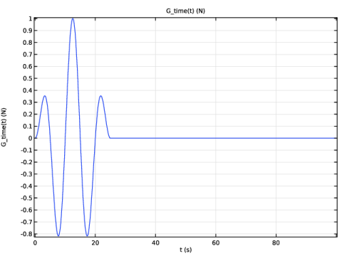
Locate the Definition section. In the Expression text field, type if(t<2.5*T0,sin(2*pi*f0*t)*sin(2*pi*f0*t/5),0).
|
|
5
|
|
6
|
Locate the Units section. In the table, enter the following settings:
|
|
7
|
|
8
|
Locate the Plot Parameters section. In the table, enter the following settings:
|
|
9
|
Click
|
|
1
|
|
2
|
|
3
|
|
4
|
Click
|
|
5
|
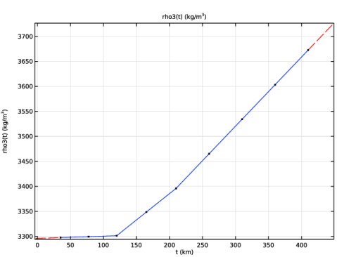
Browse to the model’s Application Libraries folder and double-click the file seismic_waves_earth_rho3.txt.
|
|
6
|
|
7
|
|
8
|
In the Function table, enter the following settings:
|
|
9
|
Click
|
|
1
|
|
2
|
|
3
|
|
4
|
Click
|
|
5
|
Click
|
|
6
|
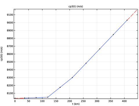
Browse to the model’s Application Libraries folder and double-click the file seismic_waves_earth_cp3.txt.
|
|
7
|
|
8
|
Click
|
|
1
|
|
2
|
|
3
|
|
4
|
Click
|
|
5
|
Click
|
|
6
|
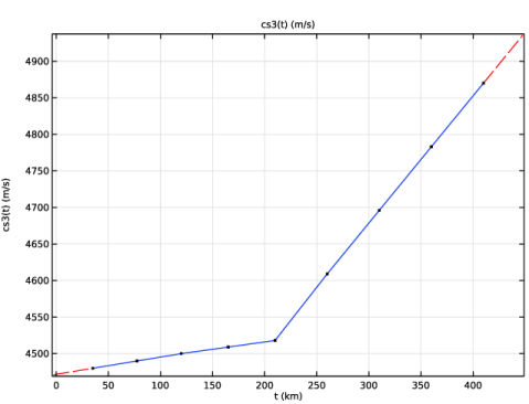
Browse to the model’s Application Libraries folder and double-click the file seismic_waves_earth_cs3.txt.
|
|
7
|
Click
|
|
1
|
|
2
|
|
3
|
|
4
|
Click
|
|
5
|
Click
|
|
6
|
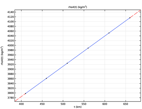
Browse to the model’s Application Libraries folder and double-click the file seismic_waves_earth_rho4.txt.
|
|
7
|
|
8
|
Click
|
|
1
|
|
2
|
|
3
|
|
4
|
Click
|
|
5
|
Click
|
|
6
|
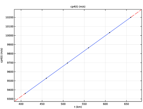
Browse to the model’s Application Libraries folder and double-click the file seismic_waves_earth_cp4.txt.
|
|
7
|
|
8
|
Click
|
|
1
|
|
2
|
|
3
|
|
4
|
Click
|
|
5
|
Click
|
|
6
|
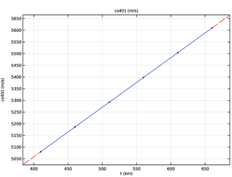
Browse to the model’s Application Libraries folder and double-click the file seismic_waves_earth_cs4.txt.
|
|
7
|
|
8
|
Click
|
|
1
|
|
2
|
|
3
|
|
4
|
Click
|
|
5
|
Click
|
|
6
|
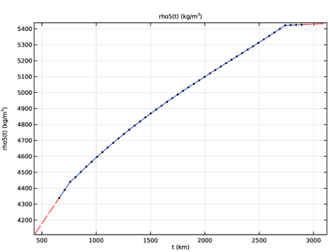
Browse to the model’s Application Libraries folder and double-click the file seismic_waves_earth_rho5.txt.
|
|
7
|
|
8
|
Click
|
|
1
|
|
2
|
|
3
|
|
4
|
Click
|
|
5
|
Click
|
|
6
|
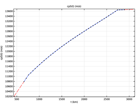
Browse to the model’s Application Libraries folder and double-click the file seismic_waves_earth_cp5.txt.
|
|
7
|
|
8
|
Click
|
|
1
|
|
2
|
|
3
|
|
4
|
Click
|
|
5
|
Click
|
|
6
|
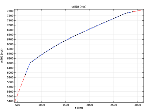
Browse to the model’s Application Libraries folder and double-click the file seismic_waves_earth_cs5.txt.
|
|
7
|
|
8
|
Click
|
|
1
|
|
2
|
|
3
|
|
4
|
Click
|
|
5
|
Click
|
|
6
|
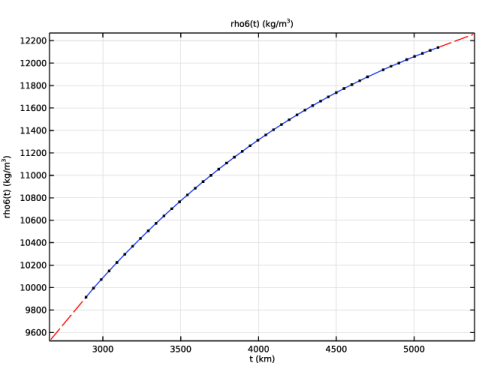
Browse to the model’s Application Libraries folder and double-click the file seismic_waves_earth_rho6.txt.
|
|
7
|
|
8
|
Click
|
|
1
|
|
2
|
|
3
|
|
4
|
Click
|
|
5
|
Click
|
|
6
|
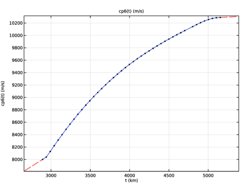
Browse to the model’s Application Libraries folder and double-click the file seismic_waves_earth_cp6.txt.
|
|
7
|
|
8
|
Click
|
|
1
|
|
2
|
|
3
|
|
4
|
Click
|
|
5
|
Click
|
|
6
|
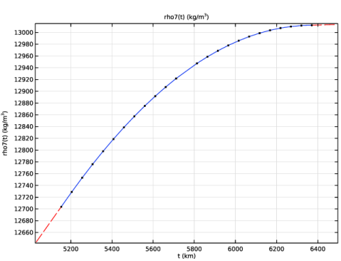
Browse to the model’s Application Libraries folder and double-click the file seismic_waves_earth_rho7.txt.
|
|
7
|
|
8
|
Click
|
|
1
|
|
2
|
|
3
|
|
4
|
Click
|
|
5
|
Click
|
|
6
|
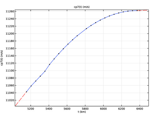
Browse to the model’s Application Libraries folder and double-click the file seismic_waves_earth_cp7.txt.
|
|
7
|
|
8
|
Click
|
|
1
|
|
2
|
|
3
|
|
4
|
Click
|
|
5
|
Click
|
|
6
|
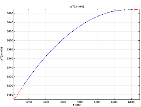
Browse to the model’s Application Libraries folder and double-click the file seismic_waves_earth_cs7.txt.
|
|
7
|
|
8
|
Click
|
|
1
|
In the Model Builder window, under Global Definitions, Ctrl-click to select Rho Layer 3 (rho3), Cp Layer 3 (cp3), and Cs Layer 3 (cs3).
|
|
2
|
Right-click and choose Group.
|
|
1
|
In the Model Builder window, under Global Definitions, Ctrl-click to select Rho Layer 4 (rho4), Cp Layer 4 (cp4), and Cs Layer 4 (cs4).
|
|
2
|
Right-click and choose Group.
|
|
1
|
In the Model Builder window, under Global Definitions, Ctrl-click to select Rho Layer 5 (rho5), Cp Layer 5 (cp5), and Cs Layer 5 (cs5).
|
|
2
|
Right-click and choose Group.
|
|
1
|
In the Model Builder window, under Global Definitions, Ctrl-click to select Rho Layer 6 (rho6) and Cp Layer 6 (cp6).
|
|
2
|
Right-click and choose Group.
|
|
1
|
In the Model Builder window, under Global Definitions, Ctrl-click to select Rho Layer 7 (rho7), Cp Layer 7 (cp7), and Cs Layer 7 (cs7).
|
|
2
|
Right-click and choose Group.
|
|
1
|
|
2
|
|
3
|
|
1
|
|
2
|
|
3
|
|
4
|
|
5
|
|
6
|
Click to expand the Layers section. In the table, enter the following settings:
|
|
7
|
Click
|
|
8
|
|
1
|
|
2
|
|
3
|
|
4
|
|
5
|
Click
|
|
1
|
|
2
|
|
3
|
|
4
|
|
5
|
Click
|
|
1
|
In the Model Builder window, under Component 1 (comp1) right-click Definitions and choose Variables.
|
|
2
|
|
1
|
|
2
|
|
3
|
|
5
|
|
6
|
|
7
|
|
1
|
|
2
|
|
3
|
|
5
|
|
6
|
|
1
|
|
2
|
|
3
|
|
4
|
|
1
|
In the Model Builder window, under Component 1 (comp1) click Pressure Acoustics, Time Explicit (pate).
|
|
2
|
|
3
|
Click
|
|
1
|
|
1
|
In the Model Builder window, under Component 1 (comp1) > Elastic Waves, Time Explicit (elte) click Elastic Waves, Time Explicit Model 1.
|
|
2
|
In the Settings window for Elastic Waves, Time Explicit Model, locate the Linear Elastic Material section.
|
|
3
|
|
1
|
|
3
|
|
4
|
|
5
|
|
1
|
|
1
|
In the Model Builder window, under Component 1 (comp1) right-click Materials and choose Blank Material.
|
|
2
|
|
3
|
|
5
|
Locate the Material Contents section. In the table, enter the following settings:
|
|
1
|
|
2
|
|
3
|
|
5
|
Locate the Material Contents section. In the table, enter the following settings:
|
|
1
|
|
2
|
|
3
|
|
5
|
Locate the Material Contents section. In the table, enter the following settings:
|
|
1
|
|
2
|
|
3
|
|
5
|
Locate the Material Contents section. In the table, enter the following settings:
|
|
1
|
|
2
|
|
3
|
|
5
|
Locate the Material Contents section. In the table, enter the following settings:
|
|
1
|
|
2
|
|
4
|
Locate the Material Contents section. In the table, enter the following settings:
|
|
1
|
In the Model Builder window, under Component 1 (comp1) > Materials right-click Layer 5 (mat5) and choose Duplicate.
|
|
2
|
|
3
|
|
5
|
Locate the Material Contents section. In the table, enter the following settings:
|
|
1
|
|
2
|
|
3
|
|
5
|
Locate the Material Contents section. In the table, enter the following settings:
|
|
1
|
In the Physics toolbar, click
|
|
1
|
|
2
|
|
3
|
|
1
|
|
2
|
|
3
|
Click the Custom button.
|
|
4
|
Locate the Element Size Parameters section.
|
|
5
|
|
6
|
|
7
|
Click
|
|
1
|
|
2
|
|
3
|
|
1
|
|
2
|
|
1
|
|
2
|
|
3
|
|
5
|
|
6
|
Locate the Element Size Parameters section.
|
|
7
|
|
1
|
|
2
|
|
3
|
|
5
|
|
6
|
Locate the Element Size Parameters section.
|
|
7
|
Select the Maximum element size checkbox. In the associated text field, type cs4(th1+th2+th3)/f0/1.5.
|
|
1
|
|
2
|
|
3
|
|
5
|
|
6
|
Locate the Element Size Parameters section.
|
|
7
|
Select the Maximum element size checkbox. In the associated text field, type cs5(th1+th2+th3+th4)/f0/1.5.
|
|
1
|
|
2
|
|
3
|
|
5
|
|
6
|
Locate the Element Size Parameters section.
|
|
7
|
Select the Maximum element size checkbox. In the associated text field, type cp6(th1+th2+th3+th4+th5)/f0/1.5.
|
|
1
|
|
2
|
|
3
|
|
5
|
|
6
|
Locate the Element Size Parameters section.
|
|
7
|
Select the Maximum element size checkbox. In the associated text field, type cs7(th1+th2+th3+th4+th5+th6)/f0/1.5.
|
|
1
|
|
2
|
|
3
|
|
5
|
|
6
|
Locate the Element Size Parameters section.
|
|
7
|
|
8
|
Click
|
|
1
|
|
2
|
|
3
|
|
4
|
|
5
|
|
6
|
Clear the Generate default plots checkbox.
|
|
7
|
Clear the Generate convergence plots checkbox.
|
|
8
|
|
1
|
|
2
|
|
3
|
|
1
|
In the Model Builder window, under Results > Datasets right-click Study 1/Solution 1 (sol1) and choose Duplicate.
|
|
1
|
|
2
|
|
3
|
|
1
|
|
2
|
|
3
|
|
1
|
|
2
|
|
3
|
|
4
|
|
1
|
|
2
|
|
3
|
|
4
|
|
5
|
|
1
|
|
2
|
Go to the Result Templates window.
|
|
3
|
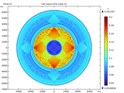
In the tree, select Study 1/Solution 1 (1) (sol1) > Acoustic–Structure Boundary, Time Explicit 1 > Cell Wave Time Scale (asbte1).
|
|
4
|
Click the Add Result Template button in the window toolbar.
|
|
5
|
|
1
|
|
2
|
|
3
|
|
4
|
|
5
|
Select the Show units checkbox.
|
|
6
|
|
7
|
|
1
|
|
2
|
|
3
|
|
4
|
|
5
|
|
1
|
|
2
|
Go to the Result Templates window.
|
|
3
|
In the tree, select Study 1/Solution 1 (1) (sol1) > Elastic Waves, Time Explicit > Velocity Magnitude (elte).
|
|
4
|
Click the Add Result Template button in the window toolbar.
|
|
5
|
|
1
|
|
2
|
|
1
|
|
2
|
|
3
|
|
4
|
Locate the Expression section. In the Expression text field, type if(isnan(pate.v_inst),elte.vel,pate.v_inst).
|
|
5
|
|
6
|
|
7
|
|
8
|
|
9
|
|
10
|
|
11
|
|
12
|
|
13
|
|
1
|
|
2
|
|
3
|
|
1
|
|
2
|
|
3
|
|
4
|
|
5
|
|
6
|
|
7
|
|
1
|
|
2
|
|
3
|
|
4
|
|
5
|
|
6
|
|
7
|
|
8
|
|
9
|
|
10
|
|
11
|
|
1
|
|
3
|
|
4
|
Clear the Evaluate the start cap checkbox.
|
|
5
|
Clear the Evaluate the end cap checkbox.
|
|
1
|
|
2
|
|
3
|
|
4
|
|
5
|
|
6
|
|
7
|
|
8
|
|
9
|
|
10
|
|
11
|
|
12
|
|
1
|
|
2
|
|
3
|
|
4
|
|
5
|
|
1
|
|
2
|
|
3
|
|
4
|
|
1
|
|
2
|
|
3
|
|
4
|
|
5
|
|
6
|
|
7
|
|
8
|
|
9
|
|
10
|
|
11
|
Click Define custom colors.
|
|
13
|
Click Add to custom colors.
|
|
14
|
|
15
|
Clear the Color legend checkbox.
|
|
1
|
|
2
|
|
3
|
|
4
|
|
5
|
|
1
|
|
2
|
|
3
|
|
4
|
|
1
|
|
2
|
|
3
|
|
1
|
In the Model Builder window, expand the Study 1 > Solver Configurations > Solution 1 (sol1) node, then click Dependent Variables 1.
|
|
2
|
|
3
|
|
4
|
In the Model Builder window, expand the Study 1 > Solver Configurations > Solution 1 (sol1) > Dependent Variables 1 node, then click Eigenvalues, Structural (comp1.asbte1.eig).
|
|
5
|
|
6
|
|
7
|
|
8
|
|
9
|
|
10
|
|
11
|
|
12
|
|
13
|
|
14
|
|
15
|
|
16
|
|
17
|
|
18
|
|
19
|
|
20
|
|
21
|
|
22
|
|
23
|
|
24
|
|
25
|
|
26
|
|
27
|
|
1
|
|
2
|
|
3
|
Select the Plot checkbox.
|
|
5
|
|
1
|
|
2
|
|
3
|
|
4
|
|
5
|
|
6
|
|
7
|
|
8
|
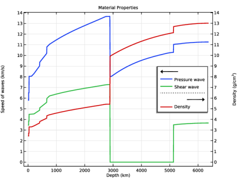
Select the Secondary y-axis label checkbox. In the associated text field, type Density (g/cm<sup>3</sup>).
|
|
9
|
|
1
|
|
3
|
|
4
|
|
5
|
|
6
|
|
7
|
|
8
|
|
9
|
|
10
|
|
11
|
|
13
|
|
14
|
|
15
|
|
16
|
|
1
|
|
2
|
|
3
|
|
4
|
Locate the Legends section. In the table, enter the following settings:
|
|
1
|
|
2
|
|
3
|
|
4
|
|
5
|
|
6
|
Locate the Legends section. In the table, enter the following settings:
|
|
1
|
|
2
|
|
3
|
Select the Plot on secondary y-axis checkbox.
|
|
4
|
|
5
|
|
1
|
|
2
|
|
3
|
|
4
|
|
1
|
|
2
|
|
1
|
|
2
|
|
3
|
|
4
|
|
1
|
|
2
|
|
3
|
|
4
|
|
1
|
|
2
|
|
3
|
|
4
|