PDF

Porous Absorber
Introduction
This is a model of acoustic absorption by a porous acoustic open cell foam. In porous materials the sound propagates in a network of small interconnected pores. Because the dimensions of the pores are small, losses occur due to thermal conduction and viscous friction. Acoustic foams are used to sound proof rooms and ducts as well as to treat reverberation problems in rooms (see Ref. 1).
The aim of the model is to characterize the absorption properties — more specifically, the specific surface impedance and the absorption coefficient — of a layer of melamine foam in terms of sound incidence angle and frequency. The melamine foam contains a solid inclusion. Inclusions are used in periodic configurations to improve absorption, in this model it is not optimized in any way. An analytical solution exists in the case where the layer is uniform. The model uses a 2D geometry of such a system and the Periodic Port to model the incident and reflected waves.
Model Definition
Figure 1 depicts the geometry of the modeled system, in which an incident sound field hits the solid-backed porous melamine-foam layer at angle θ0. A solid inclusion, circular domain of radius a, is present in the porous layer. The thickness of the porous melamine layer is Hp = 10 cm and the height of the modeled air region is H = 30 cm. In the figure, the dotted lined indicates the boundaries of the model domain. You only model a portion of width W and apply periodic Floquet boundary conditions (Periodic Condition) on the left and right boundaries to extend the domain to infinity. The incident field is modeled using the Periodic Port boundary condition. The port defines an incident plane wave at the given angle of incidence. The Periodic Port and Diffraction Order Port subfeatures combine to give a perfect non-reflecting condition for the outgoing waves.
Model the melamine foam using the Pressure Acoustics interface’s Poroacoustics domain feature using the Johnson–Champoux–Allard (JCA) model with a rigid frame. This is an equivalent fluid model for a rigid framed porous material, a so-called five parameter semi-empirical equivalent fluid model. See About the Poroacoustics Models in the Acoustics Module User’s Guide. The surrounding fluid is air, and the material parameters for the foam are as listed in Table 1 (following Ref. 2, material sample number 31).
εp
Rf
Lth
470 μm
Lv
240 μm
τ
Figure 1: Geometry of the modeled system, the air inclusion has a radius a.
The incident background pressure field is given as
(1)
where θ0 is the incidence angle and k0 is the wave number in the free field (air domain). The field is automatically defined by the Periodic Port and the associated wave vector k is picked up by the Periodic Condition.
Two parameters that characterize the absorption properties of the porous absorber are the specific normal surface impedance Z and the absorption coefficient α (see Ref. 1). The absorption coefficient, which represents the ratio of the absorbed and incident energy, is for a plane wave defined as
(2)
where R is the pressure reflection coefficient that gives the ratio of the scattered to the incident pressure. This expression is valid as long as there are no higher-order diffraction modes; higher-order modes start to occur at a given cutoff frequency. The Periodic Port defines variables exist for the scattered (outgoing) pressure acpr.pport1.p_out and the incident pressure acpr.pport1.p_in. These represent the plane wave components.
In general the absorption coefficient can be defined through its energetic definitions as
(3)
where Pscat is the total scattered power and Pinc is the total incident power. Both of these quantities are defined by the periodic port. The incident power is acpr.pport1.P_in and the total scattered power is acpr.pport1.P_out_tot. The total power variable is the sum of the scattered plane wave power and all diffraction orders included in the model.
The surface specific normal impedance (normalized by the plane wave characteristic impedance) is defined as
(4)
where ρ is the density of air, c is the speed of sound, and uu ⋅ n is the normal velocity at the surface of the melamine layer. When computing the expression it will be taken as the average at the surface of the porous layer. When averaging it is important to average the ratio p/un and not average p and un separately, the latter leads to incorrect results.
Both the absorption coefficient and the surface normal impedance are dependent on frequency and on the incidence angle.
Uniform Porous Layer Solution
In the case of a uniform porous layer (with no air inclusions) of thickness Hp backed by a sound hard wall, an analytical solution exists for the surface impedance, reflection coefficient, and absorption coefficient (see Ref. 1). The surface normal impedance (normalized by the characteristic plane wave impedance) is given by
(5)
where a subscript “c” represents complex-valued specific characteristic impedance and wave number variables from the Poroacoustic domain. From the normal impedance the analytical expression for the absorption coefficient is deduced.
Diffraction Order Ports
By itself the Periodic Port only works as a plane wave reflection condition (specular reflections). To capture the total acoustic field add the necessary Diffraction Order Port subfeatures. To assess how many are needed analyze the model at the highest frequency and evaluate the imaginary part of the mode wave numbers. This is done in the Evaluation Group in the model. Make sure to include enough modes such that all modes have a non-zero imaginary part. This means that the last included diffraction order mode is non-propagating. Note that diffraction order mode m = 0 is the specular reflection, and it is already handled by the main Periodic Port feature.
Results and Discussion
Figure 2 and Figure 3 plot the acoustic pressure fields at the frequency f = 10 kHz and incidence angles of 0° and 45° respectively. Notice how the wave is absorbed in the porous layer. Figure 4 shows the sound pressure level (SPL) for the last case.
Figure 2: Acoustic pressure field for an incidence angle of 0o and frequency f = 10 kHz.
Figure 3: Acoustic pressure for an incidence angle of 0o and frequency f = 10 kHz.
Figure 4: Sound pressure level for an incidence angle of 0o and frequency f = 10 kHz.
Figure 5 depicts the acoustic pressure (the real part) at the surface of the porous melamine layer for two angles of incidence. Figure 6 plots the specific acoustic impedance at the surface of the porous absorber (computed as the average across the surface). Figure 7 shows the absorption coefficient; comparing the energy based absorption coefficient (Equation 3) to the coefficient computed based on the reflection coefficient (Equation 2), and the analytical solution of a uniform porous layer. Finally, Figure 8 depicts the absorption coefficient for normal incidence in octave and 1/3 octave bands. The Octave Band plot feature automatically creates tables, which can be found under Results > Tables and easily exported as text or spreadsheet files.
Looking closely at Figure 7, it can be seen that the absorption coefficient based on the reflection coefficient, which assumes pure plane waves, start to differ slightly from the energy based values, at specific frequencies (1000 Hz and 1700 Hz, depending on the incidence angle). These are the cut on/off frequencies for higher order diffraction modes. In this particular setup, the difference is not large as the properties of the air inclusion are relatively close to the porous material. For other configurations, for example, having solid inclusions, the difference could be larger. The energy based absorption coefficient represents the actual absorbed energy metric.
The dependency of the surface specific impedance and/or absorption coefficient on incidence angle and frequency is important for modeling absorbers as impedance boundary conditions in, for example, a Ray Acoustics model. In larger model systems the present model could be used as a “submodel” to determine appropriate impedance boundary conditions. The real part of the impedance (the resistance) is associated with energy loss whereas the imaginary part (the reactance) is associated with phase changes of the field. The reciprocal value of the impedance is the admittance.
In this system, the absorption coefficient approaches 1 for increasing frequency. This corresponds to the frequency where the product between the porous absorber height Hp and kyπ1 of the incident wave is equal to one. This is where half a wavelength fits into the absorbing layer.
Finally, Figure 9 shows the power associated with the different diffraction order modes for the two angles of incidence. Notice the cutoff frequency for the different modes. It is also interesting to see that for the current configuration the power in the diffraction orders is comparable to the power associated with the plane-wave component.
Figure 5: Sound pressure level at the surface of the porous absorber.
Figure 6: Specific acoustic impedance at the surface of the porous absorber.
Figure 7: Absorption coefficient for the porous melamine absorber as function of frequency and incidence angle. Compared to the reflection coefficient based expression and the analytical solution of a uniform layer.
Figure 8: Absorption coefficient of the porous melamine absorber for normal incidence in octave bands, 1/3 octave bands, and continuous frequency.
Figure 9: Power (in dB) associated with the different diffraction order modes for the two angles of incidence.
Notes About the COMSOL Implementation
Periodic Floquet boundary condition
Apply a periodic Floquet boundary condition to model an infinite periodic structure. The periodicity is determined by the wave number of the background (incident) pressure field. The relation between the pressure at the left and right boundaries of the model domain is
(6)
where d = (W, 0) is a vector extending from the left to the right boundary and k is the wave vector defined in Equation 1. COMSOL Multiphysics automatically calculates the vector d when applying the Floquet periodicity.
Visualize periodic solution
To visualize the periodic solution, create an Array 2D dataset and enable Floquet–Bloch periodicity under Advanced section. Enter the same Wave vector as used in the periodic conditions.
Comparing to the Analytical Solution
In the results section the simulated absorption coefficient and surface impedance are compared to the analytical solution of a uniform porous layer. To make a verification of the model simply select the inclusion (the circular air domain) as a Poroacoustic domain and run the model again. You will find that the analytical and model results show perfect agreement.
References
1. T.J. Cox and P. D’Antonio, Acoustic Absorbers and Diffusers, Theory, Design and Applications, 2nd ed., Taylor and Francis, 2009.
2. N. Kino and T. Ueno, “Comparison between characteristic lengths and fiber equivalent diameter in glass fiber and melamine foam materials of similar flow resistivity,” J. App. Acoustics, vol. 69, pp. 325–331, 2008.
Application Library path: Acoustics_Module/Building_and_Room_Acoustics/porous_absorber
Modeling Instructions
From the File menu, choose New.
New
In the New window, click  Model Wizard.
Model Wizard
1
In the Model Wizard window, click  2D.
2
In the Select Physics tree, select Acoustics > Pressure Acoustics > Pressure Acoustics, Frequency Domain (acpr).
3
Click Add.
4
Click  Study.
5
In the Select Study tree, select General Studies > Frequency Domain.
6
Global Definitions
Load the parameters for the model. The list of parameters include geometry definitions, definitions used in the mesh, and material parameters for the melamine foam.
Parameters 1
1
In the Model Builder window, under Global Definitions click Parameters 1.
2
In the Settings window for Parameters, locate the Parameters section.
3
Click  Load from File.
4
Geometry 1
Rectangle 1 (r1)
1
In the Geometry toolbar, click  Rectangle.
2
In the Settings window for Rectangle, locate the Size and Shape section.
3
In the Width text field, type W.
4
In the Height text field, type H+Hp.
5
Locate the Position section. In the y text field, type 0.
6
In the y text field, type -Hp.
7
Click to expand the Layers section. In the table, enter the following settings:
Circle 1 (c1)
1
In the Geometry toolbar, click  Circle.
2
In the Settings window for Circle, locate the Size and Shape section.
3
In the Radius text field, type a.
4
Locate the Position section. In the x text field, type W/2.
5
In the y text field, type -Hp/2.
Difference 1 (dif1)
1
In the Geometry toolbar, click  Booleans and Partitions and choose Difference.
2
3
In the Settings window for Difference, locate the Difference section.
4
Click to select the  Activate Selection toggle button for Objects to subtract.
5
6
Click  Build All Objects.
7
Click the  Zoom Extents button in the Graphics toolbar.
The geometry should look like that in the figure below.
Definitions
Load the expressions defining the surface impedance and absorption coefficient, see Equation 2 and Equation 4, from a file.
Variables 1 - Z and alpha
1
In the Definitions toolbar, click  Local Variables.
2
In the Settings window for Variables, type Variables 1 - Z and alpha in the Label text field.
3
Locate the Variables section. Click  Load from File.
4
Load the expressions defining the analytical expressions for a single porous uniform layer with a sound hard backing, see Equation 5.
Variables 2 - Analytical
1
In the Definitions toolbar, click  Local Variables.
2
In the Settings window for Variables, type Variables 2 - Analytical in the Label text field.
3
Locate the Variables section. Click  Load from File.
4
Define two nonlocal integration couplings that act on points in the geometry. You will use them later to map (or probe) values from these points. One in the porous domain and one in the air domain.
Integration 1 (intop1)
1
In the Definitions toolbar, click  Nonlocal Couplings and choose Integration.
2
In the Settings window for Integration, locate the Source Selection section.
3
From the Geometric entity level list, choose Point.
4
Integration 2 (intop2)
1
In the Definitions toolbar, click  Nonlocal Couplings and choose Integration.
2
In the Settings window for Integration, locate the Source Selection section.
3
From the Geometric entity level list, choose Point.
4
Define an average and integration coupling on the periodic port and one on the porous-air interface. They will help compute the average reflection coefficient as well as incident and reflected powers.
Average 1 (aveop1)
1
In the Definitions toolbar, click  Nonlocal Couplings and choose Average.
2
In the Settings window for Average, locate the Source Selection section.
3
From the Geometric entity level list, choose Boundary.
4
Average 2 (aveop2)
1
In the Definitions toolbar, click  Nonlocal Couplings and choose Average.
2
In the Settings window for Average, locate the Source Selection section.
3
From the Geometric entity level list, choose Boundary.
4
Now proceed to set up the material properties. Add air as the default domain material and create a new material to define the melamine foam porosity.
Add Material
1
In the Materials toolbar, click  Add Material to open the Add Material window.
2
Go to the Add Material window.
3
In the tree, select Built-in > Air.
4
Click the Add to Component button in the window toolbar.
5
In the Materials toolbar, click  Add Material to close the Add Material window.
Materials
Melamine Foam
1
In the Model Builder window, under Component 1 (comp1) right-click Materials and choose Blank Material.
2
In the Settings window for Material, type Melamine Foam in the Label text field.
3
4
Click to expand the Material Properties section. In the Material properties tree, select Basic Properties > Porosity.
5
Click  Add to Material.
6
Locate the Material Contents section. In the table, enter the following settings:
7
Locate the Material Properties section. In the Material properties tree, select Acoustics > Poroacoustics Model > Thermal characteristic length (Lth).
8
Click  Add to Material.
9
Locate the Material Contents section. In the table, enter the following settings:
Notice that the parameter for the tortuosity is called tau0, not to be confused with the material property of the static viscous tortuosity.
Now set up the physics and the boundary conditions.
Pressure Acoustics, Frequency Domain (acpr)
Poroacoustics 1
1
In the Physics toolbar, click  Domains and choose Poroacoustics.
2
3
In the Settings window for Poroacoustics, locate the Poroacoustics Model section.
4
From the Poroacoustics model list, choose Johnson–Champoux–Allard (JCA).
5
Locate the Fluid Properties section. From the Fluid material list, choose Air (mat1).
Periodic Condition 1
1
In the Physics toolbar, click  Boundaries and choose Periodic Condition.
2
3
In the Settings window for Periodic Condition, locate the Periodicity Settings section.
4
From the Type of periodicity list, choose Floquet periodicity.
Come back and select the k-vector from the Periodic Port after defining it.
Periodic Port 1
1
In the Physics toolbar, click  Boundaries and choose Periodic Port.
2
3
In the Settings window for Periodic Port, locate the Port Mode Settings section.
4
In the Apin text field, type 1.
5
In the θin text field, type theta0.
Proceed and add the necessary number of Diffraction Order Port subfeatures. In this model the diffraction orders m from -10 to 6 are needed. This is discussed in the model documentation.
Diffraction Order Port 1
1
In the Physics toolbar, click  Attributes and choose Diffraction Order Port.
2
In the Settings window for Diffraction Order Port, locate the Diffraction Order Port section.
3
In the m text field, type -1.
Periodic Port 1
In the Model Builder window, click Periodic Port 1.
Diffraction Order Port 2
1
In the Physics toolbar, click  Attributes and choose Diffraction Order Port.
2
In the Settings window for Diffraction Order Port, locate the Diffraction Order Port section.
3
In the m text field, type -2.
Repeat this step for the remaining diffraction orders m, such that all from -10 to 6 are included.
Now all the necessary diffraction orders are included to get the full expansion at the periodic port. Make the final setting on the periodic condition.
Periodic Condition 1
1
In the Model Builder window, under Component 1 (comp1) > Pressure Acoustics, Frequency Domain (acpr) click Periodic Condition 1.
2
In the Settings window for Periodic Condition, locate the Periodicity Settings section.
3
From the kF list, choose Periodic port Floquet wave number vector (acpr/pport1).
Mesh 1
Identical Mesh 1
1
In the Mesh toolbar, click  More Attributes and choose Identical Mesh.
2
3
In the Settings window for Identical Mesh, locate the Second Entity Group section.
4
Click to select the  Activate Selection toggle button.
5
Free Triangular 1
1
In the Mesh toolbar, click  Free Triangular.
2
In the Settings window for Free Triangular, locate the Domain Selection section.
3
From the Geometric entity level list, choose Domain.
4
Size
1
In the Model Builder window, click Size.
2
In the Settings window for Size, locate the Element Size section.
3
Click the Custom button.
4
Locate the Element Size Parameters section. In the Maximum element size text field, type lambda_min/5.
This mesh resolves the smallest wavelength of the study lambda_min with 5 elements.
Mapped 1
1
In the Mesh toolbar, click  Mapped.
2
In the Settings window for Mapped, click  Build All.
3
In the Model Builder window, click Mesh 1.
Study 1
Step 1: Frequency Domain
1
In the Model Builder window, under Study 1 click Step 1: Frequency Domain.
2
In the Settings window for Frequency Domain, locate the Study Settings section.
3
Click  Range.
4
In the Range dialog, choose ISO preferred frequencies from the Entry method list.
5
In the Start frequency text field, type 10.
6
In the Stop frequency text field, type 800.
7
From the Interval list, choose 1/3 octave.
8
Click Replace.
9
In the Settings window for Frequency Domain, locate the Study Settings section.
10
Click  Range.
11
In the Range dialog, type 825 in the Start frequency text field.
12
In the Stop frequency text field, type 10000.
13
From the Interval list, choose 1/24 octave.
14
Click Add.
This frequency request uses ISO preferred sequences with a third octave spacing for low frequencies and a 24th octave spacing at higher frequencies. Add a parametric sweep over the incidence angle theta0 for the values 0o and 45o.
Parametric Sweep
1
In the Study toolbar, click  Parametric Sweep.
2
In the Settings window for Parametric Sweep, locate the Study Settings section.
3
4
5
In the Study toolbar, click  Compute.
Create an array dataset that will help you plot the Floquet periodic solution on several unit cells.
Results
Array 2D 1
1
In the Results toolbar, click  More Datasets and choose Array 2D.
2
In the Settings window for Array 2D, locate the Data section.
3
From the Dataset list, choose Study 1/Parametric Solutions 1 (sol2).
4
Locate the Array Size section. In the X size text field, type 4.
Enable Floquet-Bloch periodicity and enter the Wave vector to visualize the periodic solution.
5
Click to expand the Advanced section. Select the Floquet–Bloch periodicity checkbox.
6
Find the Wave vector subsection. In the X text field, type kx.
7
In the Y text field, type ky.
Acoustic Pressure
1
In the Model Builder window, under Results click Acoustic Pressure (acpr).
2
In the Settings window for 2D Plot Group, type Acoustic Pressure in the Label text field.
3
Locate the Data section. From the Dataset list, choose Array 2D 1.
Surface 1
1
In the Model Builder window, expand the Acoustic Pressure node, then click Surface 1.
2
In the Acoustic Pressure toolbar, click  Plot.
3
Click the  Zoom Extents button in the Graphics toolbar.
Compare the resulting plot with that in Figure 3.
Now change the incidence angle from 45o to 0o.
Acoustic Pressure
1
In the Model Builder window, click Acoustic Pressure.
2
In the Settings window for 2D Plot Group, locate the Data section.
3
From the Parameter value (theta0 (deg)) list, choose 0.
4
In the Acoustic Pressure toolbar, click  Plot.
5
Click the  Zoom Extents button in the Graphics toolbar.
The result should look like that in the following figure.
Sound Pressure Level
1
In the Model Builder window, under Results click Sound Pressure Level (acpr).
2
In the Settings window for 2D Plot Group, type Sound Pressure Level in the Label text field.
3
Locate the Data section. From the Dataset list, choose Array 2D 1.
Next, create 1D plots to depict the absorption properties of the melamine absorber.
First, reproduce the plot in Figure 5, which shows the acoustic pressure at the surface of the porous melamine layer.
Point Pressure
1
In the Results toolbar, click  1D Plot Group.
2
In the Settings window for 1D Plot Group, type Point Pressure in the Label text field.
3
Locate the Data section. From the Dataset list, choose Study 1/Parametric Solutions 1 (sol2).
4
Click to expand the Title section. From the Title type list, choose Label.
Point Graph 1
1
Right-click Point Pressure and choose Point Graph.
2
3
In the Settings window for Point Graph, click to expand the Legends section.
4
Select the Show legends checkbox.
5
In the Point Pressure toolbar, click  Plot.
6
Click the  x-Axis Log Scale button in the Graphics toolbar.
Proceed by plotting the acoustic normal impedance at the surface of the porous melamine layer. The plot should look like that in Figure 6.
Normal Impedance
1
In the Results toolbar, click  1D Plot Group.
2
In the Settings window for 1D Plot Group, type Normal Impedance in the Label text field.
3
Locate the Data section. From the Dataset list, choose Study 1/Parametric Solutions 1 (sol2).
4
Locate the Title section. From the Title type list, choose Label.
5
Locate the Plot Settings section.
6
Select the x-axis label checkbox. In the associated text field, type f (Hz).
7
Select the y-axis label checkbox. In the associated text field, type Z/(rho*c) (1).
8
Locate the Legend section. From the Position list, choose Upper right.
Global 1
1
Right-click Normal Impedance and choose Global.
2
In the Settings window for Global, locate the y-Axis Data section.
3
4
Click to expand the Legends section. In the Normal Impedance toolbar, click  Plot.
5
Click the  x-Axis Log Scale button in the Graphics toolbar.
Plot the absorption coefficient of the porous melamine layer for the two studied incidence angles (Figure 7).
Absorption Coefficient
1
In the Results toolbar, click  1D Plot Group.
2
In the Settings window for 1D Plot Group, type Absorption Coefficient in the Label text field.
3
Locate the Data section. From the Dataset list, choose Study 1/Parametric Solutions 1 (sol2).
4
Locate the Title section. From the Title type list, choose Label.
5
Locate the Plot Settings section.
6
Select the x-axis label checkbox. In the associated text field, type f (Hz).
7
Select the y-axis label checkbox. In the associated text field, type \alpha (1).
8
Locate the Legend section. From the Position list, choose Lower right.
Global 1
1
Right-click Absorption Coefficient and choose Global.
2
In the Settings window for Global, locate the y-Axis Data section.
3
4
In the Absorption Coefficient toolbar, click  Plot.
5
Click the  x-Axis Log Scale button in the Graphics toolbar.
Next, plot the absorption coefficient of the porous melamine layer for normal incidence in octave and 1/3 octave bands (Figure 8).
Normal Incidence Absorption
1
In the Results toolbar, click  1D Plot Group.
2
In the Settings window for 1D Plot Group, type Normal Incidence Absorption in the Label text field.
3
Locate the Data section. From the Dataset list, choose Study 1/Parametric Solutions 1 (sol2).
4
From the Parameter selection (theta0) list, choose From list.
5
In the Parameter values (theta0 (deg)) list box, select 0.
6
Click to expand the Title section. From the Title type list, choose Label.
7
Locate the Plot Settings section.
8
Select the x-axis label checkbox. In the associated text field, type f (Hz).
9
Select the y-axis label checkbox. In the associated text field, type \alpha (1).
10
Locate the Axis section. Select the x-axis log scale checkbox.
11
Locate the Legend section. Clear the Show legends checkbox.
Octave Band 1
1
In the Normal Incidence Absorption toolbar, click  More Plots and choose Octave Band.
2
In the Settings window for Octave Band, locate the Selection section.
3
From the Geometric entity level list, choose Global.
4
Locate the y-Axis Data section. In the Expression text field, type alpha.
5
From the Expression type list, choose General (non-dB).
6
Locate the Plot section. From the Quantity list, choose Band average power spectral density.
Octave Band 2
1
Right-click Octave Band 1 and choose Duplicate.
2
In the Settings window for Octave Band, locate the Plot section.
3
From the Band type list, choose 1/3 octave.
Octave Band 3
1
Right-click Octave Band 2 and choose Duplicate.
2
In the Settings window for Octave Band, locate the Plot section.
3
From the Quantity list, choose Continuous power spectral density.
4
Click to expand the Coloring and Style section. From the Width list, choose 2.
5
In the Normal Incidence Absorption toolbar, click  Plot.
The final two plots and evaluation group are used to assess how many diffraction order ports are needed for the given frequency range and angles of incidence.
Powers of Outgoing Modes - 0 deg
1
In the Results toolbar, click  1D Plot Group.
2
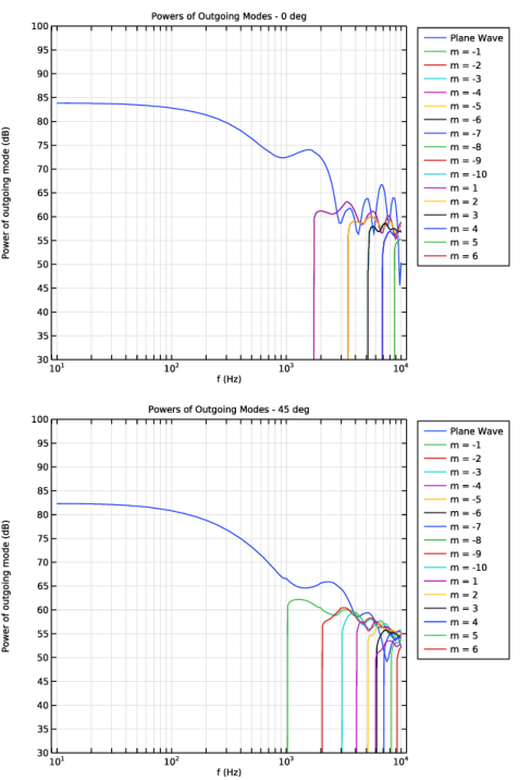
In the Settings window for 1D Plot Group, type Powers of Outgoing Modes - 0 deg in the Label text field.
3
Locate the Data section. From the Dataset list, choose Study 1/Parametric Solutions 1 (sol2).
4
From the Parameter selection (theta0) list, choose First.
5
Click to expand the Title section. From the Title type list, choose Label.
6
Locate the Plot Settings section.
7
Select the x-axis label checkbox. In the associated text field, type f (Hz).
8
Select the y-axis label checkbox. In the associated text field, type Power of outgoing mode (dB).
9
Locate the Axis section. Select the x-axis log scale checkbox.
10
Locate the Legend section. From the Layout list, choose Outside graph axis area.
Global 1
1
Right-click Powers of Outgoing Modes - 0 deg and choose Global.
2
In the Settings window for Global, locate the y-Axis Data section.
3
4
Click to expand the Legends section. Find the Include subsection. Clear the Solution checkbox.
5
In the Powers of Outgoing Modes - 0 deg toolbar, click  Plot.
Powers of Outgoing Modes - 0 deg
1
In the Model Builder window, click Powers of Outgoing Modes - 0 deg.
2
In the Settings window for 1D Plot Group, locate the Axis section.
3
Select the Manual axis limits checkbox.
4
In the y minimum text field, type 30.
5
In the y maximum text field, type 100.
6
In the Powers of Outgoing Modes - 0 deg toolbar, click  Plot.
This plot shows the power in the different diffraction order modes at 0 deg. incidence. At frequencies above 2000 Hz several modes become important, comparable to the plane wave mode.
Powers of Outgoing Modes - 45 deg
1
Right-click Powers of Outgoing Modes - 0 deg and choose Duplicate.
2
In the Settings window for 1D Plot Group, type Powers of Outgoing Modes - 45 deg in the Label text field.
3
Locate the Data section. From the Parameter selection (theta0) list, choose Last.
4
In the Powers of Outgoing Modes - 45 deg toolbar, click  Plot.
This plot shows the power in the different diffraction order modes at 45 deg. incidence. At frequencies above 1000 Hz several modes become important, comparable to the plane wave mode.
Evaluation Group 1 - Diffraction Order
1
In the Results toolbar, click  Evaluation Group.
2
In the Settings window for Evaluation Group, type Evaluation Group 1 - Diffraction Order in the Label text field.
3
Locate the Data section. From the Dataset list, choose Study 1/Parametric Solutions 1 (sol2).
4
From the Parameter selection (freq) list, choose Last.
5
Locate the Transformation section. Select the Transpose checkbox.
6
Click to expand the Format section. From the Include parameters list, choose On.
Global Evaluation 1
1
Right-click Evaluation Group 1 - Diffraction Order and choose Global Evaluation.
2
In the Settings window for Global Evaluation, locate the Expressions section.
3
4
In the Evaluation Group 1 - Diffraction Order toolbar, click  Evaluate.
This evaluation performed at the highest study frequency can be used to see when enough diffraction order ports have been added. As soon as the imaginary part of the port wave number is no longer 0, it becomes non-propagating. This happens, for the two angles if incidence combined, at m = -10 and m = 6. This analysis depends on the angle of incidence and should be done at the highest frequency.