|
|
|

|
1
|
|
2
|
In the Select Physics tree, select Acoustics > Aeroacoustics > Linearized Euler, Frequency Domain (lef).
|
|
3
|
Click Add.
|
|
4
|
|
5
|
Click Add.
|
|
6
|
Click
|
|
7
|
|
8
|
Click
|
|
1
|
|
2
|
|
3
|
Click
|
|
4
|
Browse to the model’s Application Libraries folder and double-click the file point_source_2d_jet_parameters.txt.
|
|
5
|
|
1
|
|
2
|
|
3
|
Click
|
|
4
|
Browse to the model’s Application Libraries folder and double-click the file point_source_2d_jet_geometry_parameters.txt.
|
|
5
|
|
1
|
|
2
|
|
3
|
|
4
|
Click
|
|
5
|
Browse to the model’s Application Libraries folder and double-click the file point_source_2d_jet_analytical.txt.
|
|
6
|
Locate the Data Column Settings section. In the table, click to select the cell at row number 1 and column number 3.
|
|
7
|
|
9
|
|
10
|
|
12
|
|
13
|
|
15
|
Locate the Interpolation and Extrapolation section. From the Interpolation list, choose Piecewise cubic.
|
|
16
|
|
1
|
|
2
|
|
3
|
|
4
|
|
5
|
|
6
|
Click to expand the Layers section. In the table, enter the following settings:
|
|
7
|
Select the Layers to the left checkbox.
|
|
8
|
Select the Layers to the right checkbox.
|
|
9
|
Clear the Layers on bottom checkbox.
|
|
10
|
Select the Layers on top checkbox.
|
|
11
|
Click
|
|
12
|
|
1
|
|
2
|
|
3
|
|
4
|
|
1
|
|
2
|
|
3
|
|
4
|
|
5
|
|
1
|
|
2
|
|
3
|
|
4
|
|
5
|
|
6
|
|
1
|
|
2
|
|
1
|
Go to the Add Material window.
|
|
2
|
|
3
|
Click the Add to Component button in the window toolbar.
|
|
4
|
|
1
|
|
2
|
|
3
|
|
1
|
|
2
|
|
3
|
|
1
|
|
2
|
|
3
|
|
4
|
|
1
|
|
2
|
|
3
|
|
1
|
In the Model Builder window, under Component 1 (comp1) right-click Definitions and choose Variables.
|
|
2
|
|
3
|
Click
|
|
4
|
Browse to the model’s Application Libraries folder and double-click the file point_source_2d_jet_variables.txt.
|
|
5
|
|
6
|
|
1
|
In the Model Builder window, under Component 1 (comp1) > Linearized Euler, Frequency Domain (lef) click Linearized Euler Model 1.
|
|
2
|
|
3
|
|
4
|
|
5
|
|
6
|
Locate the Fluid Properties section. From the ρ0 list, choose User defined. In the associated text field, type rho0.
|
|
1
|
|
2
|
|
3
|
|
1
|
|
3
|
|
4
|
|
1
|
|
2
|
In the Settings window for Linearized Euler, Transient, locate the Transient Solver Settings section.
|
|
3
|
|
1
|
In the Model Builder window, under Component 1 (comp1) > Linearized Euler, Transient (let) click Linearized Euler Model 1.
|
|
2
|
|
3
|
|
4
|
|
5
|
|
6
|
Locate the Fluid Properties section. From the ρ0 list, choose User defined. In the associated text field, type rho0.
|
|
1
|
|
2
|
|
3
|
|
1
|
|
3
|
|
4
|
|
1
|
|
1
|
|
2
|
|
3
|
|
1
|
|
2
|
|
3
|
Click the Custom button.
|
|
4
|
|
5
|
|
1
|
|
2
|
|
3
|
Click
|
|
5
|
|
6
|
Locate the Element Size Parameters section.
|
|
7
|
|
1
|
|
2
|
|
3
|
Select the Adjust edge mesh checkbox.
|
|
1
|
|
3
|
|
1
|
|
2
|
|
3
|
Clear the Generate default plots checkbox.
|
|
1
|
|
2
|
|
3
|
|
4
|
Locate the Physics and Variables Selection section. Select the Modify model configuration for study step checkbox.
|
|
5
|
In the tree, select Component 1 (comp1) > Definitions > Artificial Domains > Absorbing Layer 1 (ab1).
|
|
6
|
Click
|
|
7
|
|
8
|
|
9
|
|
1
|
|
2
|
Go to the Add Study window.
|
|
3
|
Find the Physics interfaces in study subsection. In the table, clear the Solve checkbox for Linearized Euler, Frequency Domain (lef).
|
|
4
|
|
5
|
Click the Add Study button in the window toolbar.
|
|
6
|
|
1
|
|
2
|
|
3
|
Locate the Physics and Variables Selection section. Select the Modify model configuration for study step checkbox.
|
|
4
|
In the tree, select Component 1 (comp1) > Definitions > Artificial Domains > Perfectly Matched Layer 1 (pml1).
|
|
5
|
Click
|
|
6
|
|
7
|
|
8
|
Clear the Generate default plots checkbox.
|
|
9
|
|
10
|
|
1
|
|
2
|
|
3
|
|
1
|
|
2
|
|
3
|
|
1
|
|
2
|
|
3
|
|
4
|
|
5
|
|
1
|
|
2
|
|
3
|
|
4
|
|
5
|
|
6
|
|
1
|
|
2
|
In the Settings window for Cut Line 2D, type Cut Line 2D - y=15, Frequency Domain in the Label text field.
|
|
3
|
|
4
|
|
5
|
|
6
|
|
1
|
|
2
|
In the Settings window for Cut Line 2D, type Cut Line 2D - y=15, Time Domain in the Label text field.
|
|
3
|
|
4
|
|
5
|
|
6
|
|
7
|
|
1
|
|
2
|
|
3
|
|
4
|
|
5
|
|
6
|
|
1
|
|
2
|
|
3
|
|
4
|
|
1
|
|
2
|
|
3
|
|
4
|
|
5
|
|
6
|
|
1
|
|
2
|
|
3
|
|
4
|
|
5
|
|
6
|
Clear the Color legend checkbox.
|
|
1
|
|
2
|
|
3
|
|
4
|
|
5
|
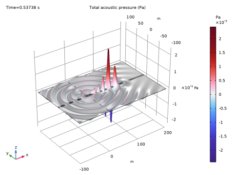
Clear the Show height axis checkbox.
|
|
6
|
|
1
|
|
2
|
|
3
|
|
4
|
|
1
|
|
2
|
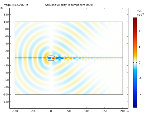
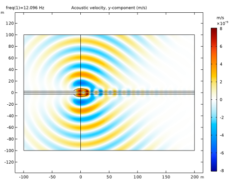
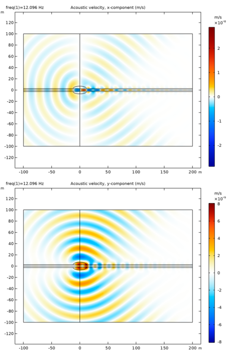
In the Settings window for Surface, click Replace Expression in the upper-right corner of the Expression section. From the menu, choose Component 1 (comp1) > Linearized Euler, Frequency Domain > Acoustic fields > Acoustic velocity - m/s > u - Acoustic velocity, x-component.
|
|
3
|
|
4
|
|
5
|
|
6
|
|
7
|
|
1
|
|
2
|
|
3
|
|
4
|
|
1
|
|
2
|
|
3
|
|
4
|
|
5
|
|
6
|
|
1
|
|
2
|
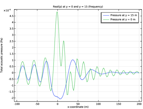
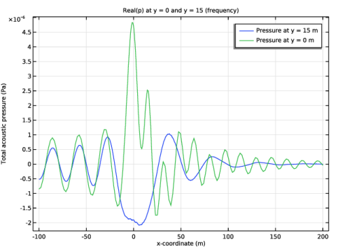
In the Settings window for 1D Plot Group, type Real(p) at y = 0 and y = 15 (frequency) in the Label text field.
|
|
3
|
|
1
|
|
2
|
|
3
|
|
4
|
|
5
|
|
6
|
|
7
|
|
8
|
|
1
|
In the Model Builder window, right-click Real(p) at y = 0 and y = 15 (frequency) and choose Line Graph.
|
|
2
|
|
3
|
Click to select the
|
|
5
|
|
6
|
|
7
|
|
8
|
|
9
|
|
11
|
|
1
|
|
2
|
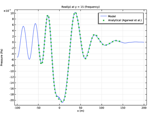
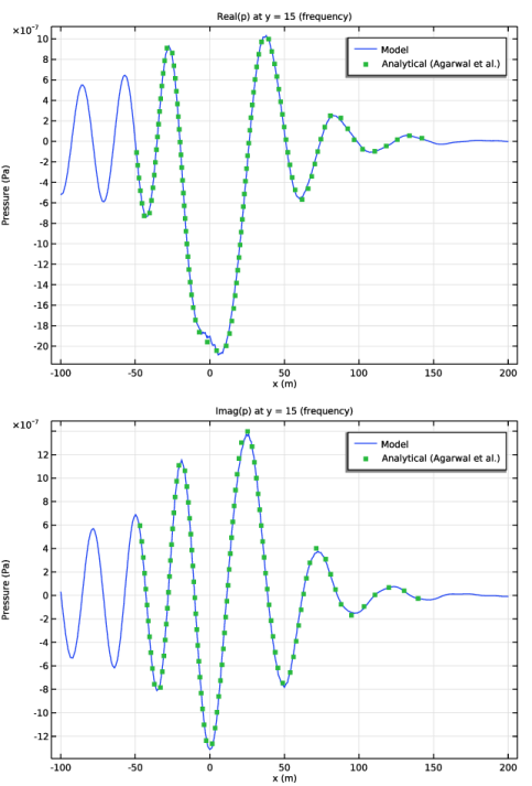
In the Settings window for 1D Plot Group, type Real(p) at y = 15 (frequency) in the Label text field.
|
|
3
|
|
4
|
|
5
|
Locate the Plot Settings section.
|
|
6
|
|
7
|
|
1
|
|
2
|
|
3
|
|
4
|
|
5
|
|
6
|
|
7
|
|
1
|
|
2
|
|
3
|
|
4
|
|
5
|
|
6
|
|
7
|
|
8
|
|
10
|
Click to expand the Coloring and Style section. Find the Line style subsection. From the Line list, choose None.
|
|
11
|
|
12
|
|
13
|
|
14
|
|
1
|
|
2
|
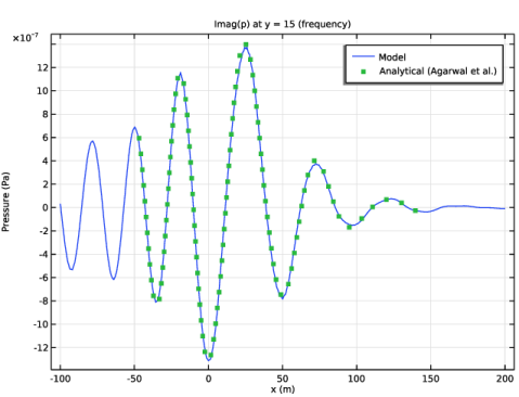
In the Settings window for 1D Plot Group, type Imag(p) at y = 15 (frequency) in the Label text field.
|
|
3
|
|
1
|
In the Model Builder window, expand the Imag(p) at y = 15 (frequency) node, then click Line Graph 1.
|
|
2
|
|
3
|
|
1
|
|
2
|
|
3
|
|
4
|
|
1
|
|
2
|
|
3
|
|
4
|
|
5
|
|
1
|
|
2
|
|
3
|
|
4
|
|
5
|
|
6
|
|
1
|
|
2
|
|
1
|
|
2
|
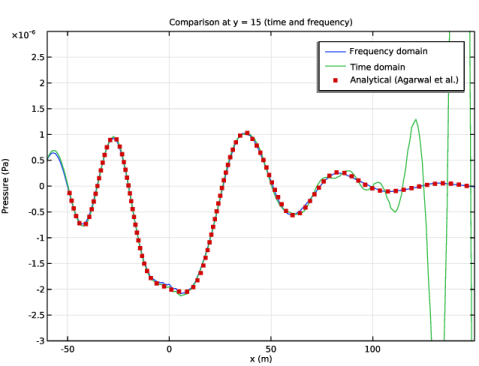
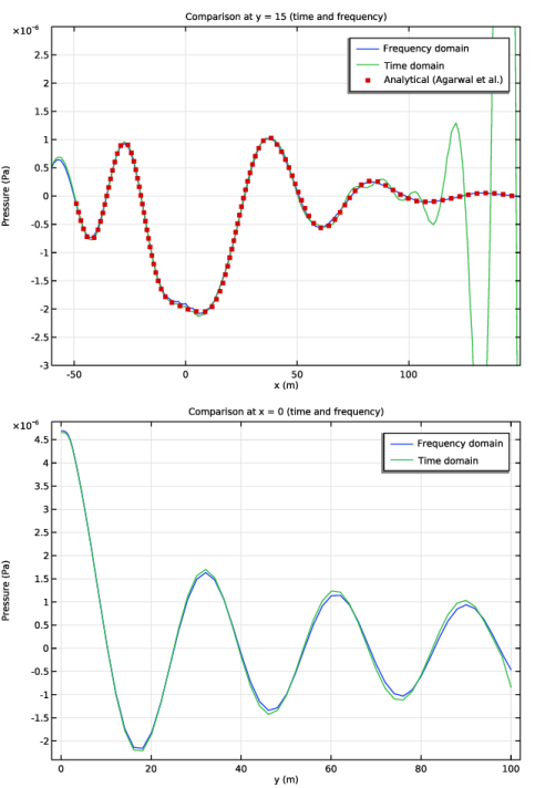
In the Settings window for 1D Plot Group, type Comparison at y = 15 (time and frequency) in the Label text field.
|
|
3
|
|
4
|
|
5
|
Locate the Plot Settings section.
|
|
6
|
|
7
|
|
1
|
|
2
|
|
3
|
|
4
|
|
5
|
|
6
|
|
7
|
|
8
|
|
10
|
|
1
|
In the Model Builder window, right-click Comparison at y = 15 (time and frequency) and choose Line Graph.
|
|
2
|
|
3
|
|
4
|
|
5
|
|
6
|
|
7
|
|
8
|
|
9
|
|
11
|
|
1
|
|
2
|
|
3
|
|
4
|
|
5
|
|
6
|
|
7
|
|
8
|
|
10
|
Click to expand the Coloring and Style section. Find the Line style subsection. From the Line list, choose None.
|
|
11
|
|
12
|
|
13
|
|
14
|
|
1
|
|
2
|
|
3
|
Select the Manual axis limits checkbox.
|
|
4
|
|
5
|
|
6
|
|
7
|
|
8
|
|
1
|
|
2
|
In the Settings window for 1D Plot Group, type Comparison at x = 0 (time and frequency) in the Label text field.
|
|
3
|
|
4
|
Locate the Plot Settings section.
|
|
5
|
|
6
|
|
1
|
|
2
|
|
3
|
Click to select the
|
|
5
|
|
6
|
|
7
|
|
8
|
|
9
|
|
1
|
In the Model Builder window, right-click Comparison at x = 0 (time and frequency) and choose Line Graph.
|
|
2
|
|
3
|
|
4
|
|
6
|
|
7
|
|
8
|
|
9
|
|
10
|
|
12
|