|
|
|
|
1
|
|
2
|
|
3
|
Click Add.
|
|
4
|
Click
|
|
5
|
In the Select Study tree, select Preset Studies for Selected Physics Interfaces > Small-Signal Analysis, Frequency Domain.
|
|
6
|
Click
|
|
1
|
|
2
|
|
3
|
|
1
|
|
2
|
|
3
|
Click
|
|
4
|
Browse to the model’s Application Libraries folder and double-click the file ow_microspeaker_parameters.txt.
|
|
1
|
|
2
|
|
3
|
|
4
|
Browse to the model’s Application Libraries folder and double-click the file ow_microspeaker_spl_39mm_test.txt.
|
|
5
|
|
6
|
|
7
|
In the Function table, enter the following settings:
|
|
8
|
Click
|
|
1
|
|
2
|
|
3
|
|
4
|
Browse to the model’s Application Libraries folder and double-click the file ow_microspeaker_bl_test.txt.
|
|
5
|
|
6
|
Locate the Interpolation and Extrapolation section. From the Interpolation list, choose Piecewise cubic.
|
|
7
|
|
8
|
|
9
|
In the Function table, enter the following settings:
|
|
10
|
Click
|
|
1
|
|
2
|
|
3
|
|
4
|
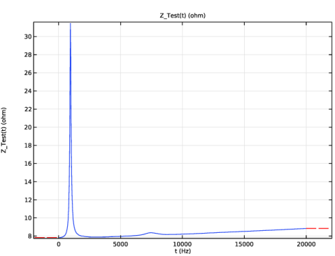
Browse to the model’s Application Libraries folder and double-click the file ow_microspeaker_z_test.txt.
|
|
5
|
|
6
|
|
7
|
In the Function table, enter the following settings:
|
|
8
|
Click
|
|
1
|
|
2
|
|
3
|
|
4
|
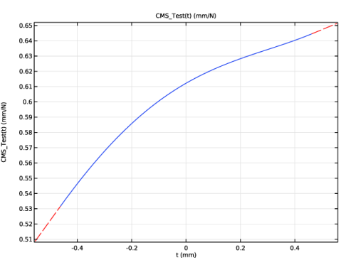
Browse to the model’s Application Libraries folder and double-click the file ow_microspeaker_cms_test.txt.
|
|
5
|
|
6
|
Locate the Interpolation and Extrapolation section. From the Interpolation list, choose Cubic spline.
|
|
7
|
|
8
|
|
9
|
In the Function table, enter the following settings:
|
|
10
|
Click
|
|
1
|
|
2
|
|
3
|
|
1
|
|
2
|
|
3
|
|
4
|
Click
|
|
5
|
Browse to the model’s Application Libraries folder and double-click the file ow_microspeaker_axisymmetric.mphbin.
|
|
6
|
Click
|
|
1
|
In the Model Builder window, under Component 1 (comp1) right-click Definitions and choose Variables.
|
|
2
|
|
3
|
Click
|
|
4
|
Browse to the model’s Application Libraries folder and double-click the file ow_microspeaker_variables_2d.txt.
|
|
1
|
|
2
|
|
3
|
|
5
|
|
6
|
Clear the Compute integral in revolved geometry checkbox.
|
|
1
|
|
2
|
Go to the Add Material window.
|
|
3
|
|
4
|
Click the Add to Component button in the window toolbar.
|
|
5
|
|
6
|
Click the Add to Component button in the window toolbar.
|
|
7
|
|
1
|
|
1
|
|
3
|
|
4
|
Click to expand the Material Properties section. In the Material properties tree, select Electromagnetic Models > Remanent Flux Density > Remanent flux density norm (normBr).
|
|
5
|
Click
|
|
6
|
Locate the Material Contents section. In the table, enter the following settings:
|
|
1
|
|
3
|
|
4
|
|
5
|
|
6
|
|
7
|
|
8
|
|
9
|
From the list, choose From diameter.
|
|
10
|
|
1
|
|
2
|
In the Settings window for Ampère’s Law in Solids, type Ampère's Law First Magnet in the Label text field.
|
|
4
|
Locate the Constitutive Relation B-H section. From the Magnetization model list, choose Remanent flux density.
|
|
5
|
Specify the e vector as
|
|
1
|
|
2
|
In the Settings window for Ampère’s Law in Solids, type Ampère's Law Second Magnet in the Label text field.
|
|
4
|
Locate the Constitutive Relation B-H section. From the Magnetization model list, choose Remanent flux density.
|
|
5
|
Specify the e vector as
|
|
1
|
|
2
|
In the Settings window for Ampère’s Law in Solids, type Ampère's Law Soft Iron in the Label text field.
|
|
4
|
|
1
|
|
3
|
|
4
|
|
1
|
|
2
|
|
3
|
From the list, choose User-controlled mesh.
|
|
1
|
|
2
|
|
3
|
Click the Custom button.
|
|
4
|
|
5
|
|
6
|
Click
|
|
1
|
|
2
|
|
3
|
|
1
|
|
2
|
|
3
|
Click the Custom button.
|
|
4
|
Locate the Element Size Parameters section.
|
|
5
|
|
6
|
Click
|
|
1
|
|
2
|
|
3
|
|
5
|
|
6
|
Locate the Element Size Parameters section.
|
|
7
|
|
8
|
Click
|
|
1
|
|
2
|
|
3
|
|
1
|
|
3
|
|
4
|
|
5
|
|
6
|
Click
|
|
1
|
|
2
|
In the Settings window for Study, type Study 1 - Axisymmetric Magnetic Analysis in the Label text field.
|
|
1
|
In the Model Builder window, under Study 1 - Axisymmetric Magnetic Analysis click Step 2: Frequency-Domain Perturbation.
|
|
2
|
|
3
|
Click
|
|
4
|
|
5
|
|
6
|
|
7
|
|
8
|
Click Replace.
|
|
9
|
|
1
|
|
2
|
|
3
|
Locate the Data section. From the Dataset list, choose Study 1 - Axisymmetric Magnetic Analysis/Solution Store 1 (sol2).
|
|
4
|
|
5
|
|
6
|
|
7
|
|
8
|
Click
|
|
1
|
|
2
|
|
3
|
|
4
|
|
5
|
Select the Secondary y-axis log scale checkbox.
|
|
6
|
|
1
|
|
2
|
|
3
|
Locate the y-Axis Data section. In the table, enter the following settings:
|
|
1
|
|
2
|
|
3
|
|
4
|
Locate the y-Axis Data section. In the table, enter the following settings:
|
|
5
|
|
1
|
|
2
|
|
3
|
|
4
|
|
5
|
|
6
|
|
7
|
|
8
|
|
9
|
|
10
|
|
11
|
|
12
|
|
13
|
|
1
|
|
2
|
|
3
|
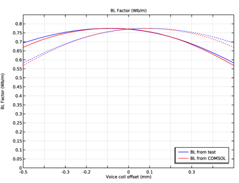
Locate the y-Axis Data section. In the Expression text field, type BL_Test(z-(-1.53[mm]-0.05[mm])/2).
|
|
4
|
|
5
|
|
6
|
|
7
|
|
8
|
|
9
|
|
10
|
|
11
|
Clear the Solution checkbox.
|
|
1
|
|
2
|
|
3
|
Locate the y-Axis Data section. In the Expression text field, type BL_Test(z-(-1.53[mm]-0.05[mm])/2).
|
|
4
|
|
5
|
|
6
|
|
7
|
|
8
|
Locate the Coloring and Style section. Find the Line style subsection. From the Line list, choose Dotted.
|
|
9
|
|
1
|
|
2
|
|
3
|
Locate the y-Axis Data section. In the Expression text field, type -int_BL(BL_integrand*coil_location_r*coil_location_z).
|
|
4
|
|
5
|
|
6
|
|
7
|
|
8
|
|
9
|
|
10
|
|
11
|
Clear the Solution checkbox.
|
|
1
|
|
2
|
|
3
|
Locate the y-Axis Data section. In the Expression text field, type -int_BL(BL_integrand*coil_location_r*coil_location_z).
|
|
4
|
|
5
|
|
6
|
|
7
|
|
8
|
|
9
|
Locate the Coloring and Style section. Find the Line style subsection. From the Line list, choose Dotted.
|
|
10
|
|
11
|
|
1
|
In the Model Builder window, under Results, Ctrl-click to select Magnetic Flux Density (mf), Magnetic Flux Density, Revolved Geometry (mf), Coil Properties from COMSOL, and BL Factor.
|
|
2
|
Right-click and choose Group.
|
|
1
|
In the Settings window for Group, type Postprocessing - Electromagnetic analysis in the Label text field.
|
|
1
|
|
2
|
In the Settings window for Evaluation Group, type Evaluation Group - Coil Properties in the Label text field.
|
|
1
|
|
2
|
|
4
|
|
1
|
|
2
|
In the Settings window for Evaluation Group, type Evaluation Group - BL Factor in the Label text field.
|
|
3
|
|
1
|
|
3
|
|
5
|
|
6
|
|
7
|
|
1
|
|
2
|
In the Settings window for Interpolation, type Coil inductance from axisymmetric model in the Label text field.
|
|
3
|
|
4
|
Locate the Data Column Settings section. In the table, click to select the cell at row number 1 and column number 1.
|
|
5
|
|
7
|
|
8
|
|
10
|
|
11
|
|
12
|
Click
|
|
1
|
|
2
|
|
1
|
|
2
|
|
3
|
|
4
|
Click
|
|
5
|
Browse to the model’s Application Libraries folder and double-click the file ow_microspeaker_geometry.mphbin.
|
|
6
|
Click
|
|
7
|
|
8
|
|
9
|
|
10
|
Clear the Automatic detection of small details checkbox.
|
|
11
|
|
1
|
In the Model Builder window, under Component 2 (comp2) right-click Definitions and choose Variables.
|
|
2
|
|
3
|
Click
|
|
4
|
Browse to the model’s Application Libraries folder and double-click the file ow_microspeaker_variables_3d.txt.
|
|
1
|
|
2
|
|
3
|
|
1
|
|
2
|
|
3
|
|
1
|
|
2
|
|
3
|
|
4
|
|
5
|
In the Add dialog, in the Selections to add list, choose Diaphragm triangular mesh and Diaphragm mapped mesh.
|
|
6
|
Click OK.
|
|
1
|
|
2
|
|
1
|
|
2
|
|
1
|
|
2
|
|
1
|
|
2
|
|
1
|
|
2
|
|
3
|
|
1
|
|
2
|
|
3
|
|
4
|
|
5
|
Click OK.
|
|
6
|
|
7
|
|
8
|
|
9
|
Click OK.
|
|
1
|
|
2
|
|
1
|
|
2
|
|
1
|
|
2
|
|
1
|
|
2
|
|
3
|
|
4
|
|
1
|
|
2
|
|
3
|
|
4
|
|
5
|
|
6
|
|
1
|
|
2
|
|
3
|
|
4
|
|
1
|
|
2
|
|
3
|
|
4
|
|
1
|
|
2
|
|
3
|
|
4
|
|
1
|
|
2
|
Go to the Add Material window.
|
|
3
|
|
4
|
Click the Add to Component button in the window toolbar.
|
|
5
|
|
1
|
In the Model Builder window, under Component 2 (comp2) right-click Materials and choose Blank Material.
|
|
2
|
|
3
|
Locate the Geometric Entity Selection section. From the Geometric entity level list, choose Boundary.
|
|
4
|
|
5
|
Locate the Material Properties section. In the Material properties tree, select Basic Properties > Density.
|
|
6
|
Click
|
|
7
|
|
8
|
Click
|
|
9
|
|
10
|
Click
|
|
11
|
|
12
|
Click
|
|
13
|
Locate the Material Contents section. In the table, enter the following settings:
|
|
1
|
|
2
|
|
3
|
|
4
|
Locate the Material Properties section. In the Material properties tree, select Basic Properties > Density.
|
|
5
|
Click
|
|
6
|
|
7
|
Click
|
|
8
|
|
9
|
Click
|
|
10
|
Locate the Material Contents section. In the table, enter the following settings:
|
|
1
|
|
2
|
Go to the Add Physics window.
|
|
3
|
Find the Physics interfaces in study subsection. In the table, clear the Solve checkbox for Study 1 - Axisymmetric Magnetic Analysis.
|
|
4
|
|
5
|
Click the Add to Component 2 button in the window toolbar.
|
|
6
|
|
7
|
|
8
|
Click the Add to Component 2 button in the window toolbar.
|
|
9
|
|
10
|
|
11
|
Click the Add to Component 2 button in the window toolbar.
|
|
12
|
|
13
|
|
14
|
Click the Add to Component 2 button in the window toolbar.
|
|
15
|
|
1
|
In the Settings window for Pressure Acoustics, Frequency Domain, locate the Domain Selection section.
|
|
2
|
|
1
|
|
2
|
|
3
|
|
4
|
Locate the Exterior Field Calculation section. From the Condition in the z = z0 plane list, choose Symmetric/Infinite sound hard boundary.
|
|
1
|
|
2
|
|
3
|
|
4
|
|
5
|
|
1
|
|
2
|
|
3
|
|
4
|
|
5
|
|
1
|
|
2
|
|
3
|
|
4
|
|
5
|
|
6
|
|
1
|
|
2
|
|
3
|
|
1
|
|
2
|
|
3
|
|
4
|
|
5
|
|
1
|
|
2
|
|
3
|
|
4
|
|
5
|
|
1
|
|
2
|
|
3
|
|
1
|
|
2
|
|
3
|
|
1
|
In the Model Builder window, under Component 2 (comp2) > Shell (shell) click Thickness and Offset 1.
|
|
2
|
|
3
|
|
4
|
|
5
|
|
1
|
|
1
|
|
2
|
|
4
|
|
1
|
|
2
|
|
4
|
|
1
|
|
2
|
|
4
|
|
1
|
|
2
|
|
3
|
|
4
|
|
5
|
|
1
|
|
2
|
|
3
|
|
4
|
|
5
|
|
1
|
In the Model Builder window, under Component 2 (comp2) right-click Multiphysics and choose Solid–Thin Structure Connection.
|
|
2
|
|
3
|
|
1
|
|
2
|
In the Settings window for Acoustic–Structure Boundary, type Acoustic-Structure Boundary - Solid in the Label text field.
|
|
3
|
|
1
|
|
2
|
In the Settings window for Acoustic–Structure Boundary, type Acoustic-Structure Boundary - Shell in the Label text field.
|
|
3
|
|
4
|
|
1
|
|
2
|
|
3
|
Click the Custom button.
|
|
4
|
|
5
|
|
6
|
|
7
|
Click
|
|
1
|
|
2
|
|
3
|
|
1
|
|
2
|
|
3
|
Click the Custom button.
|
|
4
|
Locate the Element Size Parameters section.
|
|
5
|
|
1
|
|
3
|
|
4
|
|
1
|
|
2
|
|
3
|
|
1
|
|
2
|
|
3
|
Click the Custom button.
|
|
4
|
Locate the Element Size Parameters section.
|
|
5
|
|
6
|
|
1
|
|
2
|
|
3
|
|
4
|
|
1
|
|
2
|
|
3
|
|
1
|
|
2
|
|
3
|
|
4
|
|
1
|
|
2
|
|
3
|
|
1
|
|
2
|
|
3
|
|
4
|
|
1
|
|
2
|
|
3
|
|
1
|
|
2
|
|
3
|
|
5
|
Click
|
|
1
|
|
2
|
|
3
|
|
4
|
Click
|
|
1
|
|
2
|
|
3
|
|
5
|
|
1
|
|
3
|
|
4
|
|
5
|
Click
|
|
1
|
|
2
|
Go to the Add Study window.
|
|
3
|
Find the Physics interfaces in study subsection. In the table, clear the Solve checkboxes for Magnetic Fields (mf), Pressure Acoustics, Frequency Domain (acpr), and Electrical Circuit (cir).
|
|
4
|
Find the Multiphysics couplings in study subsection. In the table, clear the Solve checkboxes for Acoustic-Structure Boundary - Solid (asb1) and Acoustic-Structure Boundary - Shell (asb2).
|
|
5
|
|
6
|
Click the Add Study button in the window toolbar.
|
|
7
|
|
1
|
|
1
|
|
2
|
|
3
|
Select the Include geometric nonlinearity checkbox.
|
|
4
|
Click to expand the Mesh Selection section. In the table, enter the following settings:
|
|
5
|
|
6
|
Click
|
|
11
|
|
12
|
|
13
|
|
14
|
|
1
|
|
2
|
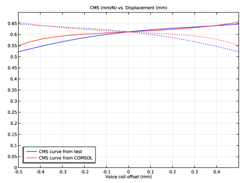
In the Settings window for Evaluation Group, type Evaluation Group - Force Displacement Curve in the Label text field.
|
|
3
|
Locate the Data section. From the Dataset list, choose Study 2 - CMS Extraction/Solution 3 (4) (sol3).
|
|
4
|
|
1
|
|
2
|
|
4
|
|
1
|
|
2
|
In the Settings window for Interpolation, type Force displacement from COMSOL in the Label text field.
|
|
3
|
|
4
|
|
5
|
Locate the Data Column Settings section. In the table, click to select the cell at row number 1 and column number 1.
|
|
6
|
|
8
|
|
9
|
|
10
|
Locate the Interpolation and Extrapolation section. From the Interpolation list, choose Piecewise cubic.
|
|
11
|
|
12
|
Click
|
|
1
|
|
1
|
|
2
|
|
3
|
|
4
|
|
5
|
|
1
|
|
2
|
|
3
|
|
4
|
|
5
|
|
6
|
|
7
|
Locate the Plot Settings section.
|
|
8
|
|
9
|
|
10
|
|
11
|
|
12
|
|
13
|
|
14
|
|
1
|
|
2
|
|
3
|
|
4
|
|
5
|
|
6
|
|
7
|
|
8
|
|
9
|
|
10
|
|
11
|
Clear the Solution checkbox.
|
|
1
|
|
2
|
|
3
|
|
4
|
Locate the Coloring and Style section. Find the Line style subsection. From the Line list, choose Dotted.
|
|
5
|
|
1
|
|
2
|
|
3
|
|
4
|
|
5
|
|
6
|
|
7
|
|
8
|
|
9
|
|
10
|
|
11
|
Clear the Solution checkbox.
|
|
1
|
|
2
|
In the Settings window for Line Graph, type CMS curve from COMSOL (inverted) in the Label text field.
|
|
3
|
|
4
|
Locate the Coloring and Style section. Find the Line style subsection. From the Line list, choose Dotted.
|
|
5
|
|
6
|
|
1
|
In the Model Builder window, under Results, Ctrl-click to select Stress (solid), Stress (shell), and CMS vs. Displacement.
|
|
2
|
Right-click and choose Group.
|
|
1
|
|
1
|
|
2
|
Go to the Add Study window.
|
|
3
|
Find the Physics interfaces in study subsection. In the table, clear the Solve checkbox for Magnetic Fields (mf).
|
|
4
|
|
5
|
Click the Add Study button in the window toolbar.
|
|
6
|
|
1
|
|
2
|
|
3
|
Click
|
|
4
|
|
5
|
|
6
|
|
7
|
|
8
|
Click Replace.
|
|
9
|
|
10
|
Select the Modify model configuration for study step checkbox.
|
|
11
|
|
12
|
Right-click and choose Disable.
|
|
13
|
Click to expand the Mesh Selection section. In the table, enter the following settings:
|
|
14
|
Right-click Study 3 - Acoustic Analysis > Step 1: Frequency Domain and choose Get Initial Value for Step.
|
|
1
|
In the Model Builder window, under Study 3 - Acoustic Analysis > Solver Configurations > Solution 4 (sol4) right-click Stationary Solver 1 and choose Fully Coupled.
|
|
2
|
Right-click Study 3 - Acoustic Analysis > Solver Configurations > Solution 4 (sol4) > Stationary Solver 1 > Suggested Iterative Solver (GMRES with Direct Precond.) (asb1_sshc1_asb2) and choose Enable.
|
|
3
|
In the Model Builder window, expand the Study 3 - Acoustic Analysis > Solver Configurations > Solution 4 (sol4) > Stationary Solver 1 > Suggested Iterative Solver (GMRES with Direct Precond.) (asb1_sshc1_asb2) node, then click Direct Preconditioner 2.
|
|
4
|
|
5
|
|
6
|
|
7
|
Click OK.
|
|
8
|
|
1
|
|
2
|
|
3
|
Click
|
|
4
|
Browse to the model’s Application Libraries folder and double-click the file ow_microspeaker_spl_39mm_thermoviscous.txt.
|
|
5
|
|
1
|
|
2
|
|
3
|
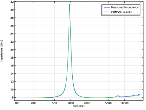
Locate the Data section. From the Dataset list, choose Study 3 - Acoustic Analysis/Solution 4 (6) (sol4).
|
|
4
|
Locate the Plot Settings section.
|
|
5
|
|
6
|
|
7
|
|
8
|
Select the y-axis log scale checkbox.
|
|
9
|
|
1
|
|
2
|
|
4
|
|
1
|
|
2
|
In the Settings window for 1D Plot Group, type Speaker Sensitivity and Phase at 39 mm in the Label text field.
|
|
3
|
Locate the Data section. From the Dataset list, choose Study 3 - Acoustic Analysis/Solution 4 (6) (sol4).
|
|
4
|
|
5
|
|
6
|
Locate the Plot Settings section.
|
|
7
|
|
8
|
|
1
|
|
2
|
|
4
|
|
1
|
|
2
|
|
3
|
|
4
|
|
5
|
|
6
|
|
7
|
|
1
|
|
2
|
|
3
|
|
4
|
|
5
|
Select the Show legends checkbox.
|
|
6
|
|
1
|
|
3
|
Select the Unwrap phase checkbox.
|
|
1
|
|
2
|
|
3
|
Select the Two y-axes checkbox.
|
|
4
|
|
5
|
Select the Secondary y-axis label checkbox.
|
|
6
|
|
7
|
|
8
|
|
9
|
|
10
|
|
11
|
Select the x-axis log scale checkbox.
|
|
12
|
|
13
|
|
14
|
|
15
|
|
1
|
|
2
|
|
3
|
Locate the Data section. From the Dataset list, choose Study 3 - Acoustic Analysis/Solution 4 (6) (sol4).
|
|
4
|
Locate the Plot Settings section.
|
|
5
|
|
6
|
|
7
|
|
1
|
|
2
|
|
4
|
|
1
|
In the Model Builder window, under Results, Ctrl-click to select Acoustic Pressure (acpr), Sound Pressure Level (acpr), Acoustic Pressure, Isosurfaces (acpr), Exterior-Field Sound Pressure Level (acpr), Exterior-Field Pressure (acpr), Exterior-Field Sound Pressure Level xy-plane (acpr), Stress (solid) 1, Stress (shell) 1, Outgoing Acoustic Energy, Speaker Sensitivity and Phase at 39 mm, and Total Impedance.
|
|
2
|
Right-click and choose Group.
|
|
1
|
|
1
|
|
2
|
|
3
|
Locate the Data section. From the Dataset list, choose Study 3 - Acoustic Analysis/Solution 4 (6) (sol4).
|
|
4
|
|
5
|
|
6
|
|
7
|
|
8
|
|
9
|
|
1
|
|
2
|
|
3
|
|
4
|
|
5
|
|
1
|
|
2
|
|
3
|
|
4
|
|
5
|
|
1
|
|
2
|
|
3
|
|
1
|
|
2
|
|
3
|
|
4
|
|
5
|
|
6
|
|
7
|
Clear the Color checkbox.
|
|
8
|
Clear the Color and data range checkbox.
|
|
9
|
Clear the Tube radius scale factor checkbox.
|
|
1
|
|
2
|
|
3
|
|
4
|
|
5
|
|
1
|
|
2
|
|
3
|
|
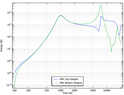
1
|
|
2
|
|
3
|
|
4
|
|
1
|
|
2
|
|
3
|
|
1
|
|
2
|
|
3
|
|
4
|
|
5
|
|
1
|
|
2
|
|
3
|
|
4
|
|
5
|
|
1
|
|
2
|