|
|
|

|
1
|
|
2
|
In the Select Physics tree, select Acoustics > Thermoviscous Acoustics > Thermoviscous Acoustics, Transient (tatd).
|
|
3
|
Click Add.
|
|
4
|
In the Select Physics tree, select Acoustics > Pressure Acoustics > Pressure Acoustics, Transient (actd).
|
|
5
|
Click Add.
|
|
6
|
Click
|
|
7
|
|
8
|
Click
|
|
1
|
|
2
|
|
3
|
|
4
|
Browse to the model’s Application Libraries folder and double-click the file nonlinear_slit_resonator_parameters_model.txt.
|
|
1
|
|
2
|
|
3
|
|
4
|
Browse to the model’s Application Libraries folder and double-click the file nonlinear_slit_resonator_parameters_geometry.txt.
|
|
1
|
|
2
|
|
3
|
|
4
|
|
5
|
|
6
|
|
1
|
|
2
|
|
3
|
|
4
|
|
5
|
|
6
|
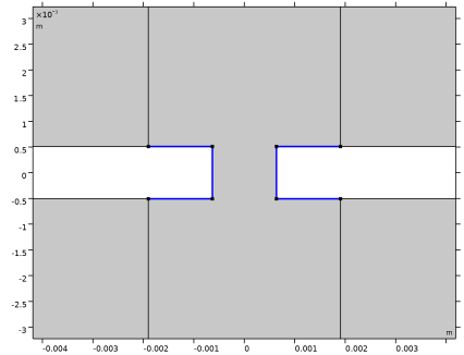
Click to expand the Layers section. In the table, enter the following settings:
|
|
7
|
Clear the Layers on bottom checkbox.
|
|
8
|
Select the Layers to the left checkbox.
|
|
9
|
Select the Layers to the right checkbox.
|
|
1
|
|
2
|
|
3
|
|
4
|
|
5
|
|
1
|
|
2
|
|
3
|
|
4
|
|
5
|
|
1
|
|
2
|
|
3
|
|
4
|
|
5
|
|
1
|
|
2
|
|
3
|
|
1
|
|
2
|
|
3
|
|
4
|
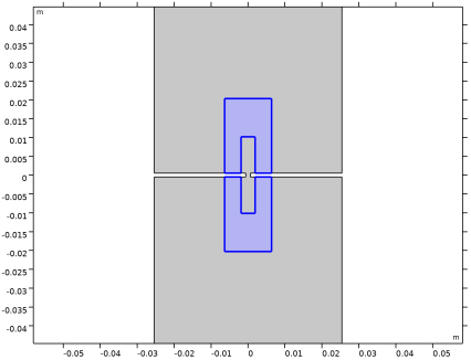
On the object uni1, select Domains 3, 7, 10, and 13–15 only.
|
|
1
|
|
2
|
On the object del1, select Boundaries 24 and 25 only.
|
|
3
|
|
1
|
|
2
|
Go to the Add Material window.
|
|
3
|
|
4
|
Click the Add to Component button in the window toolbar.
|
|
5
|
|
1
|
|
2
|
|
3
|
|
4
|
|
1
|
|
2
|
|
3
|
Click in the Graphics window and then press Ctrl+A to select all domains.
|
|
4
|
|
1
|
|
2
|
|
1
|
|
2
|
|
3
|
|
4
|
|
1
|
|
2
|
|
3
|
|
1
|
In the Model Builder window, under Component 1 (comp1) click Thermoviscous Acoustics, Transient (tatd).
|
|
2
|
|
3
|
|
4
|
|
5
|
Click to expand the Discretization section. From the Element order for velocity list, choose Linear.
|
|
6
|
|
7
|
|
8
|
|
9
|
|
10
|
Click OK.
|
|
11
|
In the Settings window for Thermoviscous Acoustics, Transient, click to expand the Stabilization section.
|
|
12
|
|
1
|
|
2
|
In the Settings window for Nonlinear Thermoviscous Acoustics Contributions, locate the Domain Selection section.
|
|
3
|
|
1
|
|
2
|
|
3
|
|
4
|
|
1
|
In the Model Builder window, expand the Component 1 (comp1) > Pressure Acoustics, Transient (actd) node, then click Pressure Acoustics, Transient (actd).
|
|
2
|
|
3
|
|
4
|
|
1
|
|
2
|
|
3
|
|
1
|
|
2
|
|
3
|
|
4
|
|
5
|
|
6
|
|
1
|
In the Physics toolbar, click
|
|
2
|
In the Settings window for Acoustic–Thermoviscous Acoustic Boundary, locate the Boundary Selection section.
|
|
3
|
|
1
|
|
2
|
|
3
|
Click the Custom button.
|
|
4
|
|
5
|
|
6
|
|
7
|
|
1
|
|
2
|
|
3
|
|
5
|
|
6
|
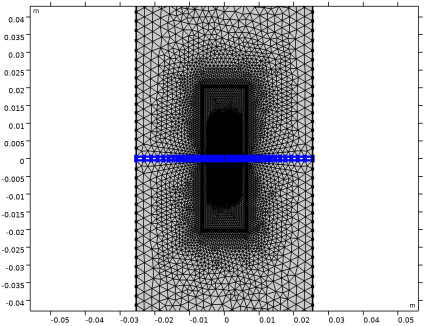
Locate the Element Size Parameters section.
|
|
7
|
|
1
|
|
2
|
|
3
|
|
5
|
|
6
|
Locate the Element Size Parameters section.
|
|
7
|
|
1
|
|
2
|
|
3
|
|
4
|
|
5
|
|
6
|
Locate the Element Size Parameters section.
|
|
7
|
|
1
|
|
2
|
|
3
|
|
5
|
|
6
|
Locate the Element Size Parameters section.
|
|
7
|
|
8
|
Click
|
|
1
|
|
2
|
|
3
|
Clear the Smooth transition to interior mesh checkbox.
|
|
1
|
|
3
|
|
4
|
|
5
|
|
6
|
|
7
|
Click
|
|
1
|
|
2
|
|
3
|
Click
|
|
1
|
|
2
|
|
3
|
|
4
|
|
1
|
|
2
|
|
3
|
|
4
|
|
5
|
|
6
|
|
1
|
|
2
|
|
3
|
|
1
|
|
2
|
|
3
|
|
4
|
|
5
|
|
1
|
|
2
|
|
3
|
|
4
|
|
5
|
|
6
|
|
1
|
|
2
|
|
1
|
|
2
|
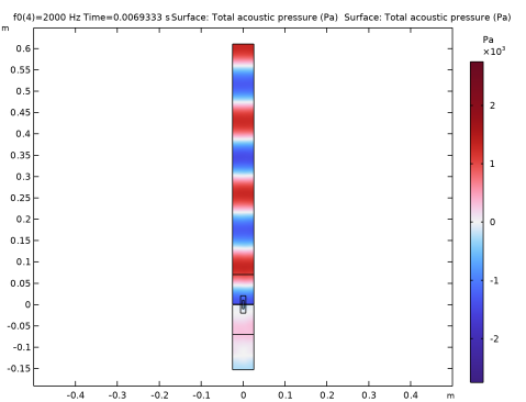
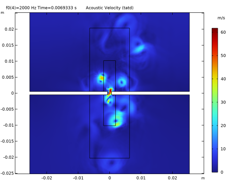
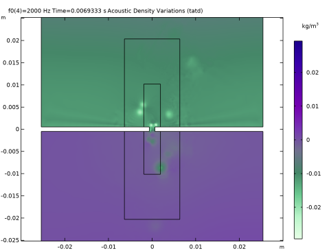
In the Settings window for 2D Plot Group, type Acoustic Density Variations (tatd) in the Label text field.
|
|
3
|
|
4
|
|
5
|
|
1
|
|
2
|
|
3
|
|
4
|
|
5
|
|
6
|
|
1
|
|
2
|
|
3
|
|
4
|
|
1
|
|
2
|
|
3
|
|
4
|
|
1
|
|
2
|
|
3
|
|
4
|
|
5
|
|
1
|
|
3
|
|
1
|
|
2
|
|
3
|
|
4
|
|
5
|
|
1
|
|
3
|
|
4
|
|
5
|
|
6
|
|
7
|
Select the Frequency range checkbox.
|
|
8
|
|
9
|
|
10
|
|
11
|
|
12
|
|
1
|
|
2
|
|
3
|
|
4
|
|
5
|
|
6
|
Locate the Plot Settings section.
|
|
7
|
|
8
|
|
1
|
|
3
|
|
4
|
|
5
|
|
6
|
|
1
|
|
3
|
|
4
|
|
5
|
|
6
|
|
8
|
|
1
|
|
2
|
|
3
|
|
4
|
|
5
|
|
6
|
Locate the Plot Settings section.
|
|
7
|
|
8
|
|
9
|
|
10
|
|
11
|
|
12
|
|
1
|
|
3
|
|
4
|
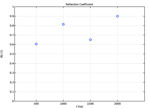
In the Expression text field, type sqrt(timeint(Tstart,Tend-T0,(actd.p_t-actd.p_i)^2))/sqrt(timeint(Tstart,Tend-T0,actd.p_i^2)).
|
|
5
|
|
6
|
|
7
|
Click to expand the Coloring and Style section. Find the Line style subsection. From the Line list, choose None.
|
|
8
|
|
9
|
|
10
|
|
1
|
|
2
|
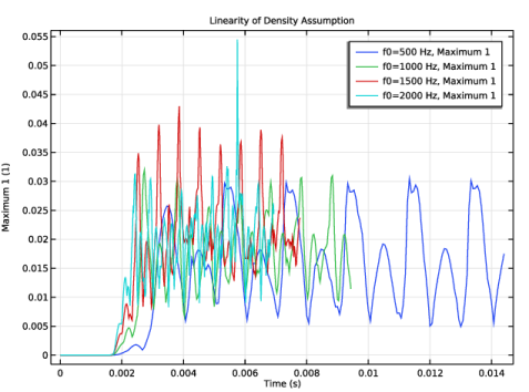
In the Settings window for 1D Plot Group, type Linearity of Density Assumption in the Label text field.
|
|
3
|
|
4
|
|
1
|
|
2
|
|
4
|