|
|
|
|
•
|
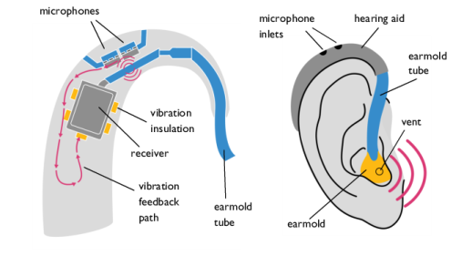
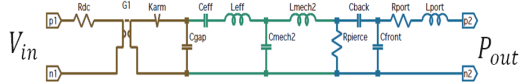
In the lumped equivalent circuit model of the receiver, the effects of variation in the skin depth of eddy currents in the steel armature is approximated by a semi-capacitor, a special component with a complex admittance proportional to the square root of iω. In the imported SPICE circuit equivalent topology network list (in the model the file lumped_receiver_vibroacoustic_TEC30033.cir is imported), the value of this component, here a resistor, is temporarily set to 1, using:
|
|
1
|
|
2
|
|
3
|
Click Add.
|
|
4
|
|
5
|
Click Add.
|
|
6
|
In the Select Physics tree, select Acoustics > Pressure Acoustics > Pressure Acoustics, Frequency Domain (acpr).
|
|
7
|
Click Add.
|
|
8
|
Click
|
|
9
|
|
10
|
Click
|
|
1
|
|
2
|
|
3
|
Click
|
|
4
|
Browse to the model’s Application Libraries folder and double-click the file lumped_receiver_vibroacoustic_parameters.txt.
|
|
1
|
|
2
|
Browse to the model’s Application Libraries folder and double-click the file lumped_receiver_vibroacoustic_geom_sequence.mph.
|
|
3
|
|
1
|
|
2
|
|
3
|
|
4
|
|
5
|
|
6
|
|
7
|
Click
|
|
1
|
|
2
|
|
3
|
|
4
|
|
5
|
Browse to the model’s Application Libraries folder and double-click the file lumped_receiver_vibroacoustic_variables_main.txt.
|
|
1
|
|
2
|
|
3
|
|
4
|
Browse to the model’s Application Libraries folder and double-click the file lumped_receiver_vibroacoustic_variables_receiver.txt.
|
|
1
|
|
2
|
|
3
|
Click
|
|
4
|
|
6
|
|
1
|
|
2
|
|
1
|
|
2
|
|
1
|
|
2
|
|
3
|
|
1
|
|
2
|
|
3
|
|
1
|
|
2
|
|
3
|
|
1
|
|
2
|
|
1
|
|
2
|
|
3
|
|
4
|
|
5
|
Click OK.
|
|
1
|
|
2
|
|
1
|
|
2
|
|
3
|
|
4
|
|
1
|
|
2
|
|
3
|
|
1
|
|
2
|
Go to the Add Material window.
|
|
3
|
|
4
|
Click the Add to Component button in the window toolbar.
|
|
1
|
|
2
|
|
1
|
|
2
|
|
3
|
|
4
|
Locate the Material Contents section. In the table, enter the following settings:
|
|
5
|
|
1
|
|
2
|
|
1
|
In the Model Builder window, under Component 1 (comp1) click Pressure Acoustics, Frequency Domain (acpr).
|
|
2
|
In the Settings window for Pressure Acoustics, Frequency Domain, locate the Domain Selection section.
|
|
3
|
|
1
|
In the Model Builder window, under Component 1 (comp1) right-click Electrical Circuit (cir) and choose Import SPICE Netlist.
|
|
2
|
Browse to the model’s Application Libraries folder and double-click the file lumped_receiver_vibroacoustic_TEC30033.cir.
|
|
1
|
In the Model Builder window, expand the Subcircuit Definition TEC30033 (TEC30033) node, then click Resistor RKARM (RKARM).
|
|
2
|
|
3
|
|
1
|
|
2
|
|
3
|
|
1
|
|
2
|
|
4
|
|
1
|
|
2
|
|
1
|
|
2
|
|
3
|
|
1
|
|
2
|
|
1
|
|
2
|
|
3
|
|
4
|
Locate the Density section. From the ρ list, choose User defined. Locate the Center of Rotation section. From the list, choose User defined.
|
|
5
|
|
1
|
|
2
|
In the Settings window for Mass and Moment of Inertia, locate the Coordinate System Selection section.
|
|
3
|
|
4
|
|
5
|
|
6
|
|
7
|
From the list, choose Symmetric.
|
|
8
|
Specify the I matrix as
|
|
1
|
|
2
|
|
3
|
|
4
|
|
5
|
|
6
|
|
1
|
|
2
|
|
3
|
|
4
|
|
1
|
|
1
|
|
3
|
|
4
|
|
1
|
In the Model Builder window, under Component 1 (comp1) > Electrical Circuit (cir) click External I vs. U 1 (IvsU1).
|
|
2
|
|
3
|
|
1
|
|
2
|
|
3
|
|
4
|
|
5
|
|
1
|
In the Physics toolbar, click
|
|
2
|
|
3
|
|
1
|
|
1
|
|
3
|
|
4
|
|
1
|
|
2
|
|
3
|
Click the Custom button.
|
|
4
|
|
5
|
|
1
|
|
2
|
|
3
|
|
1
|
|
2
|
|
3
|
Click the Custom button.
|
|
4
|
Locate the Element Size Parameters section.
|
|
5
|
|
1
|
|
2
|
|
1
|
|
2
|
|
3
|
Click
|
|
4
|
|
5
|
|
6
|
|
7
|
|
8
|
Click Replace.
|
|
9
|
|
1
|
|
1
|
|
2
|
|
3
|
|
4
|
|
1
|
|
2
|
|
1
|
|
2
|
|
3
|
|
4
|
|
5
|
|
6
|
|
1
|
|
2
|
|
3
|
|
4
|
|
5
|
|
6
|
|
7
|
|
8
|
|
9
|
|
1
|
In the Model Builder window, expand the Acoustic Pressure, Isosurfaces (acpr) node, then click Isosurface 1.
|
|
2
|
|
3
|
|
1
|
|
2
|
|
3
|
|
1
|
In the Acoustic Pressure, Isosurfaces (acpr) toolbar, click
|
|
2
|
|
3
|
|
4
|
Locate the Positioning section. Find the x grid points subsection. From the Entry method list, choose Coordinates.
|
|
5
|
|
6
|
|
7
|
|
8
|
|
9
|
|
10
|
|
1
|
|
2
|
|
3
|
|
4
|
Click
|
|
5
|
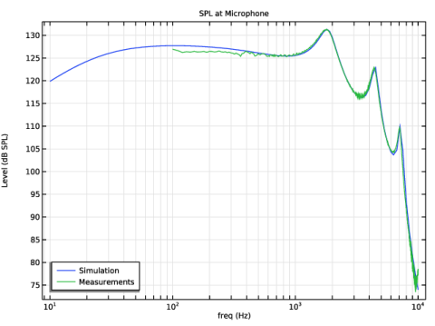
Browse to the model’s Application Libraries folder and double-click the file lumped_receiver_vibroacoustic_SPL_data.txt.
|
|
6
|
Click
|
|
7
|
Locate the Data Column Settings section. In the table, click to select the cell at row number 2 and column number 1.
|
|
8
|
|
1
|
|
2
|
|
3
|
|
4
|
Click
|
|
5
|
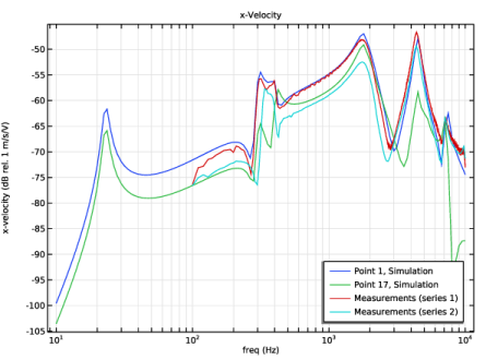
Browse to the model’s Application Libraries folder and double-click the file lumped_receiver_vibroacoustic_xvel_data_01.txt.
|
|
6
|
Click
|
|
7
|
Locate the Data Column Settings section. In the table, enter the following settings:
|
|
8
|
|
10
|
|
1
|
|
2
|
|
3
|
|
4
|
Click
|
|
5
|
Browse to the model’s Application Libraries folder and double-click the file lumped_receiver_vibroacoustic_xvel_data_02.txt.
|
|
6
|
Click
|
|
7
|
|
1
|
|
2
|
|
3
|
|
4
|
Click
|
|
5
|
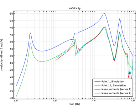
Browse to the model’s Application Libraries folder and double-click the file lumped_receiver_vibroacoustic_zvel_data_01.txt.
|
|
6
|
Click
|
|
7
|
Locate the Data Column Settings section. In the table, enter the following settings:
|
|
8
|
|
10
|
|
1
|
|
2
|
|
3
|
|
4
|
Click
|
|
5
|
Browse to the model’s Application Libraries folder and double-click the file lumped_receiver_vibroacoustic_zvel_data_02.txt.
|
|
6
|
Click
|
|
7
|
|
1
|
|
2
|
|
3
|
|
4
|
|
5
|
|
6
|
|
7
|
|
1
|
|
2
|
|
3
|
|
4
|
Locate the Plot Settings section.
|
|
5
|
|
6
|
|
7
|
|
1
|
|
2
|
|
1
|
|
2
|
|
3
|
|
4
|
|
5
|
|
6
|
|
7
|
|
8
|
|
9
|
|
11
|
|
1
|
|
2
|
|
3
|
|
4
|
Locate the Plot Settings section.
|
|
5
|
|
6
|
|
7
|
|
1
|
|
3
|
|
4
|
|
5
|
|
6
|
|
7
|
|
1
|
|
2
|
|
3
|
|
4
|
Locate the y-Axis Data section. In the Expression text field, type 20*log10(sqrt(xvel_real_01(f)^2+xvel_imag_01(f)^2)).
|
|
5
|
|
6
|
|
7
|
|
8
|
|
9
|
|
1
|
|
2
|
|
3
|
|
4
|
Locate the Legends section. In the table, enter the following settings:
|
|
5
|
|
1
|
|
2
|
|
3
|
|
4
|
Locate the Plot Settings section.
|
|
5
|
|
6
|
|
1
|
|
3
|
|
4
|
|
5
|
|
1
|
|
2
|
|
3
|
|
4
|
Locate the Plot Settings section.
|
|
5
|
|
6
|
|
7
|
|
1
|
|
3
|
|
4
|
|
5
|
|
6
|
|
7
|
|
1
|
|
2
|
|
3
|
|
4
|
Locate the y-Axis Data section. In the Expression text field, type 20*log10(sqrt(zvel_real_01(f)^2+zvel_imag_01(f)^2)).
|
|
5
|
|
6
|
|
7
|
|
8
|
|
9
|
|
1
|
|
2
|
|
3
|
|
4
|
Locate the Legends section. In the table, enter the following settings:
|
|
5
|
|
1
|
|
2
|
|
3
|
Click
|
|
4
|
Browse to the model’s Application Libraries folder and double-click the file lumped_receiver_vibroacoustic_geom_sequence_parameters.txt.
|
|
1
|
|
2
|
|
3
|
|
4
|
|
5
|
|
6
|
|
1
|
|
2
|
|
3
|
|
4
|
|
5
|
|
6
|
|
7
|
|
1
|
|
2
|
|
3
|
|
4
|
|
5
|
|
6
|
|
7
|
|
8
|
Click to expand the Layers section. In the table, enter the following settings:
|
|
1
|
|
2
|
|
3
|
|
4
|
|
5
|
|
6
|
|
7
|
|
1
|
|
2
|
|
3
|
|
4
|
|
5
|
|
6
|
|
7
|
|
1
|
|
2
|
|
3
|
|
4
|
|
5
|
On the object cyl1, select Boundary 4 only.
|
|
1
|
|
2
|
|
3
|
|
4
|
On the object cyl3, select Boundary 3 only.
|
|
1
|
|
2
|
Select the object cyl2 only.
|
|
3
|
|
4
|
|
5
|
|
6
|
Click
|
|
1
|
|
2
|
Select the object par1 only.
|
|
3
|
|
4
|
|
5
|
Click
|
|
1
|
|
2
|
Click in the Graphics window and then press Ctrl+A to select all objects.
|
|
3
|
|
4
|
|
5
|
|
6
|
Click
|
|
1
|
|
2
|
Click in the Graphics window and then press Ctrl+A to select all objects.
|
|
3
|
|
4
|
|
5
|
|
6
|
|
7
|
|
8
|
Click
|
|
1
|
|
2
|
|
3
|