|
|
|
|
1
|
|
2
|
|
3
|
Click Add.
|
|
4
|
In the Select Physics tree, select Acoustics > Aeroacoustics > Linearized Potential Flow, Frequency Domain (lpff).
|
|
5
|
Click Add.
|
|
6
|
Click
|
|
7
|
|
8
|
Click
|
|
1
|
|
2
|
|
3
|
Click
|
|
4
|
Browse to the model’s Application Libraries folder and double-click the file generic_nacelle_liner_parameters.txt.
|
|
1
|
|
2
|
|
3
|
|
4
|
|
5
|
|
1
|
|
2
|
|
3
|
|
4
|
|
5
|
|
1
|
|
2
|
|
3
|
|
4
|
|
5
|
|
6
|
|
1
|
|
2
|
|
3
|
|
4
|
On the object pc2, select Point 1 only.
|
|
5
|
|
6
|
On the object pc1, select Point 1 only.
|
|
1
|
|
2
|
Select the object ls2 only.
|
|
3
|
|
4
|
|
5
|
Click
|
|
1
|
|
2
|
Select the object off1 only.
|
|
1
|
|
2
|
On the object ls2, select Point 1 only.
|
|
3
|
|
4
|
|
5
|
On the object off2, select Point 1 only.
|
|
1
|
|
2
|
On the object ls2, select Point 2 only.
|
|
3
|
|
4
|
|
5
|
On the object off2, select Point 2 only.
|
|
1
|
|
2
|
|
3
|
|
4
|
|
5
|
|
6
|
|
7
|
|
1
|
|
2
|
|
4
|
|
5
|
|
6
|
|
1
|
|
2
|
|
3
|
|
4
|
Click
|
|
1
|
|
2
|
|
3
|
|
4
|
|
5
|
|
6
|
|
7
|
Click to expand the Layers section. In the table, enter the following settings:
|
|
1
|
|
2
|
|
3
|
|
4
|
Click
|
|
1
|
|
2
|
|
3
|
|
4
|
On the object uni1, select Domains 1–3 and 9–11 only.
|
|
5
|
Click
|
|
1
|
|
2
|
Select the object del1 only.
|
|
3
|
|
4
|
|
5
|
Click
|
|
1
|
|
2
|
|
3
|
|
4
|
On the object mov1, select Boundary 5 only.
|
|
5
|
|
6
|
Click
|
|
1
|
|
2
|
On the object fin, select Boundary 19 only.
|
|
1
|
|
2
|
|
1
|
|
2
|
Go to the Add Material window.
|
|
3
|
|
4
|
Click the Add to Component button in the window toolbar.
|
|
5
|
|
1
|
|
2
|
|
4
|
|
5
|
|
6
|
|
8
|
|
9
|
|
10
|
|
1
|
|
2
|
|
3
|
|
1
|
|
3
|
|
4
|
|
1
|
|
1
|
In the Model Builder window, under Component 1 (comp1) click Linearized Potential Flow, Frequency Domain (lpff).
|
|
2
|
In the Settings window for Linearized Potential Flow, Frequency Domain, locate the Linearized Potential Flow Equation Settings section.
|
|
3
|
|
1
|
|
3
|
|
4
|
|
5
|
Locate the Port Incident Mode Settings section. From the Incident wave excitation at this port list, choose On.
|
|
6
|
|
7
|
Locate the Port Incident Mode Settings section. From the Define incident wave list, choose Amplitude (pressure).
|
|
8
|
|
1
|
|
3
|
|
4
|
Locate the Impedance section. From the Impedance model list, choose Brambley (finite boundary layer).
|
|
5
|
|
6
|
|
1
|
|
3
|
|
4
|
|
1
|
|
2
|
|
3
|
Click the Custom button.
|
|
4
|
|
1
|
|
2
|
|
3
|
|
5
|
Click
|
|
1
|
|
3
|
|
4
|
|
5
|
Click
|
|
1
|
|
2
|
|
1
|
|
2
|
|
3
|
|
4
|
Locate the Physics and Variables Selection section. Select the Modify model configuration for study step checkbox.
|
|
5
|
In the tree, select Component 1 (comp1) > Linearized Potential Flow, Frequency Domain (lpff) > Impedance - Brambley.
|
|
6
|
Right-click and choose Disable.
|
|
1
|
|
2
|
Go to the Add Study window.
|
|
3
|
Find the Studies subsection. In the Select Study tree, select Preset Studies for Some Physics Interfaces > Stationary.
|
|
4
|
Click the Add Study button in the window toolbar.
|
|
5
|
|
1
|
|
2
|
|
1
|
|
2
|
|
3
|
|
4
|
Click
|
|
7
|
Click
|
|
8
|
|
9
|
|
10
|
|
11
|
Click Replace.
|
|
1
|
|
2
|
|
3
|
|
4
|
|
5
|
Click Import.
|
|
6
|
Click
|
|
1
|
|
2
|
Go to the Add Material window.
|
|
3
|
|
4
|
Click the Add to Component button in the window toolbar.
|
|
5
|
|
1
|
|
2
|
Go to the Add Physics window.
|
|
3
|
|
4
|
Click the Add to Component 2 button in the window toolbar.
|
|
5
|
|
6
|
Click the Add to Component 2 button in the window toolbar.
|
|
7
|
|
8
|
Click the Add to Component 2 button in the window toolbar.
|
|
9
|
|
1
|
In the Settings window for Linearized Navier–Stokes, Boundary Mode, locate the Boundary Selection section.
|
|
2
|
Click
|
|
1
|
|
3
|
|
4
|
From the list, choose Pressure.
|
|
1
|
|
3
|
|
4
|
From the list, choose Fully developed flow.
|
|
5
|
|
6
|
|
1
|
In the Physics toolbar, click
|
|
2
|
|
3
|
|
4
|
|
1
|
|
3
|
|
4
|
|
6
|
|
7
|
|
8
|
|
1
|
|
3
|
|
4
|
|
6
|
|
7
|
|
8
|
|
1
|
In the Model Builder window, under Component 2 (comp2) click Linearized Navier–Stokes, Frequency Domain (lnsf).
|
|
2
|
In the Settings window for Linearized Navier–Stokes, Frequency Domain, locate the Linearized Navier–Stokes Equation Settings section.
|
|
3
|
Select the Out-of-plane mode extension checkbox.
|
|
4
|
|
1
|
In the Model Builder window, under Component 2 (comp2) > Linearized Navier–Stokes, Frequency Domain (lnsf) click Linearized Navier–Stokes Model 1.
|
|
2
|
|
3
|
|
1
|
|
2
|
|
3
|
|
4
|
|
1
|
|
3
|
|
4
|
|
1
|
|
3
|
In the Settings window for Background Acoustic Fields, locate the Background Acoustic Fields section.
|
|
4
|
In the pb text field, type withsol('sol8',genext1(p3)/maxop1(p3)*exp(-i*lnsbm.kn*z),setind(lambda,n+1))*p0.
|
|
5
|
|
6
|
In the Tb text field, type withsol('sol8',genext1(T2)/maxop1(p3)*exp(-i*lnsbm.kn*z),setind(lambda,n+1))*p0.
|
|
1
|
|
2
|
|
3
|
|
5
|
|
6
|
|
7
|
|
1
|
|
2
|
|
3
|
|
1
|
In the Model Builder window, under Component 2 (comp2) click Linearized Navier–Stokes, Boundary Mode (lnsbm).
|
|
2
|
In the Settings window for Linearized Navier–Stokes, Boundary Mode, locate the Linearized Navier–Stokes Equation Settings section.
|
|
3
|
Select the Out-of-plane mode extension checkbox.
|
|
4
|
|
1
|
|
2
|
Go to the Add Study window.
|
|
3
|
Find the Studies subsection. In the Select Study tree, select Preset Studies for Some Physics Interfaces > Stationary with Initialization.
|
|
4
|
Click the Add Study button in the window toolbar.
|
|
1
|
|
2
|
|
3
|
In the table, clear the Use checkboxes for Linearized Navier–Stokes, Frequency Domain (lnsf), Linearized Navier–Stokes, Boundary Mode (lnsbm), and Background Fluid Flow Coupling 1 (bffc1).
|
|
4
|
Click
|
|
5
|
Click to collapse the Sequence Type section. Click to collapse the Physics-Controlled Mesh section. Click to expand the Sequence Type section. Click to expand the Physics-Controlled Mesh section. Locate the Sequence Type section. From the list, choose User-controlled mesh.
|
|
1
|
|
2
|
Click in the Graphics window and then press Ctrl+A to select all domains.
|
|
1
|
|
2
|
Click in the Graphics window and then press Ctrl+A to select all domains.
|
|
1
|
In the Model Builder window, expand the Boundary Layers 1 node, then click Boundary Layer Properties 1.
|
|
3
|
|
4
|
|
5
|
|
1
|
|
2
|
|
1
|
|
3
|
|
4
|
|
1
|
|
2
|
|
3
|
|
1
|
|
2
|
|
3
|
|
4
|
|
5
|
|
6
|
Click
|
|
7
|
|
8
|
Click
|
|
1
|
|
2
|
|
3
|
|
1
|
|
2
|
|
3
|
In the tree, select Component 2 (comp2).
|
|
4
|
Right-click and choose Disable in Solvers.
|
|
5
|
|
1
|
In the Model Builder window, expand the Study 2 - LPFF - Brambley node, then click Step 1: Stationary.
|
|
2
|
|
3
|
|
1
|
|
2
|
|
3
|
|
4
|
|
1
|
|
2
|
In the Settings window for Wall Distance Initialization, locate the Physics and Variables Selection section.
|
|
3
|
Select the Modify model configuration for study step checkbox.
|
|
4
|
In the tree, select Component 2 (comp2) > Definitions > Artificial Domains > Perfectly Matched Layer 2 (pml2).
|
|
5
|
Right-click and choose Disable.
|
|
6
|
In the tree, select Component 2 (comp2) > Definitions > Artificial Domains > Perfectly Matched Layer 3 (pml3).
|
|
7
|
Right-click and choose Disable.
|
|
1
|
|
2
|
|
3
|
|
4
|
Select the Modify model configuration for study step checkbox.
|
|
5
|
In the tree, select Component 2 (comp2) > Definitions > Artificial Domains > Perfectly Matched Layer 2 (pml2).
|
|
6
|
Right-click and choose Disable.
|
|
7
|
In the tree, select Component 2 (comp2) > Definitions > Artificial Domains > Perfectly Matched Layer 3 (pml3).
|
|
8
|
Right-click and choose Disable.
|
|
9
|
|
1
|
Go to the Add Study window.
|
|
2
|
Find the Studies subsection. In the Select Study tree, select Preset Studies for Selected Multiphysics > Mapping.
|
|
3
|
Click the Add Study button in the window toolbar.
|
|
1
|
|
2
|
|
3
|
|
4
|
|
5
|
|
1
|
In the Model Builder window, under Component 2 (comp2) > Linearized Navier–Stokes, Boundary Mode (lnsbm) click Linearized Navier–Stokes Model 1.
|
|
2
|
|
3
|
|
4
|
|
5
|
|
1
|
|
2
|
|
3
|
|
4
|
|
1
|
|
2
|
Go to the Add Material window.
|
|
3
|
|
4
|
Click the Add to Component button in the window toolbar.
|
|
5
|
|
1
|
|
2
|
|
1
|
Go to the Add Study window.
|
|
2
|
Find the Studies subsection. In the Select Study tree, select Preset Studies for Some Physics Interfaces > Mode Analysis.
|
|
3
|
Click the Add Study button in the window toolbar.
|
|
1
|
|
2
|
|
3
|
|
4
|
Select the Search for modes around shift checkbox.
|
|
5
|
Click to expand the Values of Dependent Variables section. Find the Values of variables not solved for subsection. From the Settings list, choose User controlled.
|
|
6
|
|
7
|
|
8
|
Click to expand the Filtering and Sorting section. Find the Sorting subsection. From the Ordering list, choose Descending.
|
|
9
|
|
10
|
|
11
|
|
1
|
Go to the Add Study window.
|
|
2
|
Find the Studies subsection. In the Select Study tree, select Preset Studies for Some Physics Interfaces > Frequency Domain.
|
|
3
|
Click the Add Study button in the window toolbar.
|
|
1
|
|
2
|
|
3
|
Locate the Physics and Variables Selection section. In the Solve for column of the table, clear the checkbox for Component 1 (comp1).
|
|
4
|
Select the Modify model configuration for study step checkbox.
|
|
5
|
In the tree, select Component 2 (comp2) > Linearized Navier–Stokes, Frequency Domain (lnsf) > Impedance 1.
|
|
6
|
Right-click and choose Disable.
|
|
7
|
Click to expand the Values of Dependent Variables section. Find the Values of variables not solved for subsection. From the Settings list, choose User controlled.
|
|
8
|
|
9
|
|
10
|
|
11
|
|
12
|
|
1
|
Go to the Add Study window.
|
|
2
|
Find the Studies subsection. In the Select Study tree, select Preset Studies for Some Physics Interfaces > Frequency Domain.
|
|
3
|
Click the Add Study button in the window toolbar.
|
|
1
|
|
2
|
|
3
|
Locate the Physics and Variables Selection section. In the Solve for column of the table, clear the checkbox for Component 1 (comp1).
|
|
4
|
Locate the Values of Dependent Variables section. Find the Values of variables not solved for subsection. From the Settings list, choose User controlled.
|
|
5
|
|
6
|
|
7
|
|
8
|
|
9
|
|
1
|
In the Model Builder window, under Results, Ctrl-click to select Velocity (spf), Pressure (spf), Velocity, 3D (spf), and Wall Resolution (spf).
|
|
2
|
Right-click and choose Group.
|
|
1
|
In the Model Builder window, under Results, Ctrl-click to select Acoustic Pressure (lnsbm), Acoustic Velocity (lnsbm), Temperature Variation (lnsbm), and Background Mean Flow (lnsbm).
|
|
2
|
Right-click and choose Group.
|
|
1
|
In the Model Builder window, under Results, Ctrl-click to select Acoustic Pressure (lnsf), Acoustic Velocity (lnsf), Temperature Variation (lnsf), Background Mean Flow (lnsf), Acoustic Pressure (lnsf) 1, Acoustic Velocity (lnsf) 1, Temperature Variation (lnsf) 1, and Background Mean Flow (lnsf) 1.
|
|
2
|
Right-click and choose Group.
|
|
1
|
|
2
|
|
3
|
Select the Manual color range checkbox.
|
|
4
|
|
1
|
|
2
|
|
3
|
|
5
|
|
1
|
|
2
|
|
3
|
|
1
|
|
2
|
In the Settings window for Surface, click Replace Expression in the upper-right corner of the Expression section. From the menu, choose Component 1 (comp1) > Definitions > Perfectly Matched Layer 1 > pml1.dDist - Distance function - m.
|
|
1
|
|
2
|
|
3
|
Click Replace Expression in the upper-right corner of the Expression section. From the menu, choose Component 2 (comp2) > Definitions > Perfectly Matched Layer 2 > pml2.dDist - Distance function - m.
|
|
4
|
|
1
|
|
2
|
|
3
|
Click Replace Expression in the upper-right corner of the Expression section. From the menu, choose Component 2 (comp2) > Definitions > Perfectly Matched Layer 3 > pml3.dDist - Distance function - m.
|
|
4
|
|
5
|
|
6
|
|
7
|
|
1
|
|
2
|
|
3
|
|
4
|
Locate the Plot Settings section.
|
|
5
|
|
6
|
|
7
|
|
8
|
|
9
|
|
10
|
|
11
|
|
1
|
|
2
|
|
4
|
|
5
|
|
6
|
|
7
|
|
8
|
|
9
|
|
10
|
|
11
|
Clear the Solution checkbox.
|
|
1
|
|
2
|
|
3
|
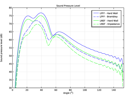
Locate the Data section. From the Dataset list, choose Study 2 - LPFF - Brambley/Solution 3 (5) (sol3).
|
|
4
|
|
5
|
|
6
|
Locate the Coloring and Style section. Find the Line style subsection. From the Line list, choose Dashed.
|
|
1
|
|
2
|
|
3
|
Locate the Data section. From the Dataset list, choose Study 6 - LNS - Hard Wall/Solution 9 (18) (sol9).
|
|
4
|
|
6
|
|
7
|
|
8
|
|
1
|
|
2
|
|
3
|
Locate the Data section. From the Dataset list, choose Study 7 - LNS - Impedance/Solution 10 (20) (sol10).
|
|
4
|
Locate the Coloring and Style section. Find the Line style subsection. From the Line list, choose Dashed.
|
|
5
|
|
1
|
|
2
|
|
3
|
Locate the Data section. From the Dataset list, choose Study 2 - LPFF - Brambley/Solution 3 (5) (sol3).
|
|
4
|
|
5
|
|
6
|
|
7
|
Locate the Plot Settings section.
|
|
8
|
|
9
|
|
1
|
|
2
|
|
4
|
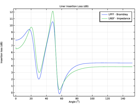
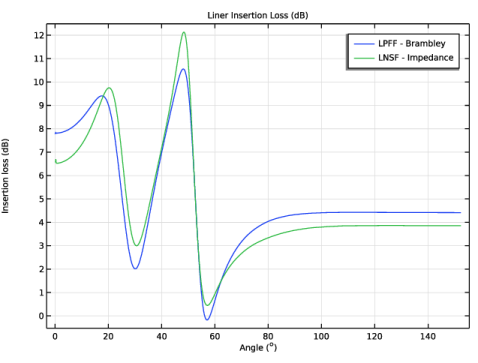
Locate the y-Axis Data section. In the Expression text field, type withsol('sol1',up(lpff.Lp))-up(lpff.Lp).
|
|
5
|
|
6
|
|
7
|
|
8
|
|
9
|
|
10
|
Clear the Solution checkbox.
|
|
1
|
|
2
|
|
3
|
Locate the Data section. From the Dataset list, choose Study 7 - LNS - Impedance/Solution 10 (20) (sol10).
|
|
4
|
|
6
|
Locate the y-Axis Data section. In the Expression text field, type withsol('sol9',up(comp2.lnsf.Lp_t))-up(comp2.lnsf.Lp_t).
|
|
7
|
|
1
|
|
2
|
|
3
|
|
4
|
Locate the Plot Settings section.
|
|
5
|
|
6
|
|
1
|
|
2
|
|
3
|
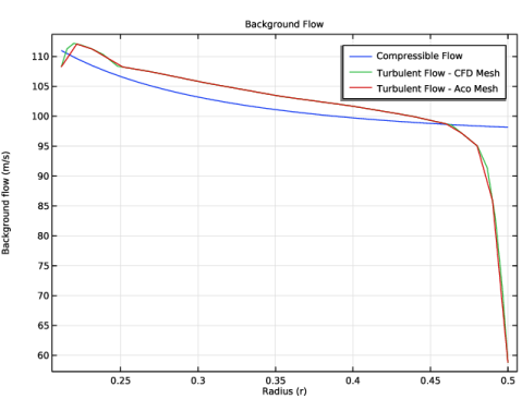
Locate the Data section. From the Dataset list, choose Study 1 - LPFF - Hard Wall/Solution 1 (1) (sol1).
|
|
5
|
Click Replace Expression in the upper-right corner of the y-Axis Data section. From the menu, choose Component 1 (comp1) > Compressible Potential Flow > cpf.normV - Velocity norm - m/s.
|
|
6
|
|
7
|
|
8
|
|
9
|
|
10
|
Clear the Solution checkbox.
|
|
1
|
|
2
|
|
3
|
|
4
|
|
6
|
Click Replace Expression in the upper-right corner of the y-Axis Data section. From the menu, choose Component 2 (comp2) > Turbulent Flow, SST > Velocity and pressure > spf.U - Velocity magnitude - m/s.
|
|
7
|
|
1
|
|
2
|
|
3
|
|
4
|
|
6
|
|
7
|