|
|
|

|
1
|
|
2
|
|
3
|
Click Add.
|
|
4
|
In the Select Physics tree, select Acoustics > Aeroacoustics > Linearized Potential Flow, Boundary Mode (lpfbm).
|
|
5
|
Click Add.
|
|
6
|
|
7
|
In the Select Physics tree, select Acoustics > Aeroacoustics > Linearized Potential Flow, Boundary Mode (lpfbm).
|
|
8
|
Click Add.
|
|
9
|
|
10
|
In the Select Physics tree, select Acoustics > Aeroacoustics > Linearized Potential Flow, Frequency Domain (lpff).
|
|
11
|
Click Add.
|
|
12
|
Click
|
|
13
|
|
14
|
Click
|
|
1
|
In the Model Builder window, click the root node.
|
|
2
|
|
3
|
|
1
|
|
2
|
|
3
|
Click
|
|
4
|
Browse to the model’s Application Libraries folder and double-click the file flow_duct_impedance_parameters.txt.
|
|
1
|
|
2
|
|
3
|
|
4
|
|
1
|
|
2
|
|
3
|
|
4
|
|
5
|
|
1
|
|
2
|
|
3
|
|
4
|
|
5
|
|
1
|
|
2
|
|
1
|
|
2
|
|
3
|
|
4
|
On the object uni1, select Point 5 only.
|
|
5
|
|
6
|
On the object pc1, select Point 1 only.
|
|
1
|
|
2
|
On the object uni1, select Point 4 only.
|
|
3
|
|
4
|
|
5
|
On the object pc1, select Point 2 only.
|
|
6
|
|
1
|
|
2
|
On the object uni1, select Boundaries 1 and 3 only.
|
|
3
|
|
1
|
|
2
|
Click in the Graphics window and then press Ctrl+D to clear all objects.
|
|
3
|
|
1
|
|
2
|
|
3
|
|
4
|
|
1
|
|
2
|
|
3
|
|
1
|
In the Model Builder window, under Component 1 (comp1) right-click Definitions and choose Variables.
|
|
2
|
|
3
|
|
5
|
Locate the Variables section. In the table, enter the following settings:
|
|
1
|
|
2
|
|
3
|
|
1
|
|
2
|
|
3
|
|
1
|
|
2
|
|
3
|
|
1
|
|
1
|
|
2
|
|
3
|
|
4
|
|
1
|
|
2
|
|
3
|
|
4
|
|
1
|
|
2
|
|
3
|
|
4
|
|
1
|
|
2
|
|
3
|
|
4
|
|
5
|
|
1
|
In the Model Builder window, under Component 1 (comp1) > Compressible Potential Flow (cpf) click Compressible Potential Flow Model 1.
|
|
2
|
In the Settings window for Compressible Potential Flow Model, locate the Compressible Potential Flow Model section.
|
|
3
|
|
1
|
|
2
|
|
3
|
|
1
|
|
2
|
|
3
|
|
1
|
In the Model Builder window, under Component 1 (comp1) click Linearized Potential Flow, Boundary Mode (lpfbm).
|
|
2
|
In the Settings window for Linearized Potential Flow, Boundary Mode, locate the Boundary Selection section.
|
|
3
|
|
4
|
|
1
|
In the Model Builder window, under Component 1 (comp1) > Linearized Potential Flow, Boundary Mode (lpfbm) click Linearized Potential Flow Model 1.
|
|
2
|
|
3
|
|
4
|
|
5
|
|
1
|
|
3
|
|
4
|
|
1
|
In the Model Builder window, under Component 1 (comp1) click Linearized Potential Flow, Boundary Mode 2 (lpfbm2).
|
|
2
|
In the Settings window for Linearized Potential Flow, Boundary Mode, locate the Boundary Selection section.
|
|
3
|
|
4
|
|
1
|
In the Model Builder window, under Component 1 (comp1) > Linearized Potential Flow, Boundary Mode 2 (lpfbm2) click Linearized Potential Flow Model 1.
|
|
2
|
|
3
|
|
4
|
|
5
|
|
1
|
|
3
|
|
4
|
|
1
|
|
2
|
|
3
|
|
1
|
|
2
|
|
3
|
Click the Custom button.
|
|
4
|
|
6
|
Locate the Element Size Parameters section.
|
|
7
|
|
1
|
|
2
|
|
3
|
Click the Custom button.
|
|
4
|
|
5
|
|
1
|
|
2
|
|
1
|
|
2
|
|
1
|
|
2
|
|
3
|
Click
|
|
5
|
|
1
|
|
2
|
|
3
|
|
4
|
|
1
|
|
2
|
|
3
|
|
4
|
|
5
|
|
1
|
|
2
|
|
3
|
|
4
|
|
5
|
|
6
|
|
1
|
|
2
|
|
3
|
|
4
|
|
5
|
|
6
|
|
7
|
|
8
|
|
9
|
|
1
|
|
2
|
|
3
|
|
4
|
|
5
|
|
6
|
|
7
|
|
8
|
|
9
|
|
1
|
|
2
|
Go to the Add Study window.
|
|
3
|
Find the Physics interfaces in study subsection. In the table, clear the Solve checkboxes for Compressible Potential Flow (cpf), Linearized Potential Flow, Boundary Mode 2 (lpfbm2), and Linearized Potential Flow, Frequency Domain (lpff).
|
|
4
|
Find the Studies subsection. In the Select Study tree, select Preset Studies for Selected Physics Interfaces > Mode Analysis.
|
|
5
|
Click the Add Study button in the window toolbar.
|
|
1
|
|
2
|
|
3
|
Click
|
|
1
|
|
2
|
|
3
|
|
4
|
|
5
|
|
6
|
|
7
|
Find the Rectangle search region subsection. In the Smallest real part (Out-of-plane wave number) text field, type -1.1*k0max_abs.
|
|
8
|
|
9
|
|
10
|
|
11
|
Click to expand the Values of Dependent Variables section. Find the Values of variables not solved for subsection. From the Settings list, choose User controlled.
|
|
12
|
|
13
|
|
14
|
|
15
|
|
1
|
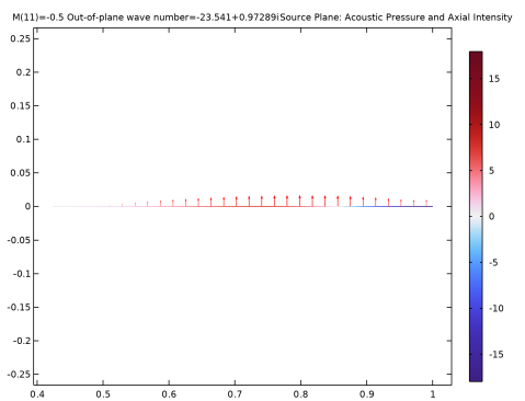
In the Settings window for 2D Plot Group, type Source Plane: Acoustic Pressure and Axial Intensity in the Label text field.
|
|
2
|
|
3
|
|
4
|
Select the Apply to dataset edges checkbox.
|
|
5
|
|
1
|
|
2
|
In the Settings window for Arrow Line, click Replace Expression in the upper-right corner of the Expression section. From the menu, choose Component 1 (comp1) > Linearized Potential Flow, Boundary Mode > Intensity > lpfbm.Ir,lpfbm.Iz - Intensity.
|
|
3
|
|
4
|
|
5
|
|
1
|
|
2
|
|
3
|
|
1
|
|
2
|
|
3
|
|
1
|
|
2
|
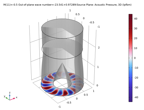
In the Settings window for 3D Plot Group, type Source Plane: Acoustic Pressure, 3D (lpfbm) in the Label text field.
|
|
3
|
|
1
|
|
2
|
|
3
|
|
4
|
|
5
|
|
6
|
|
1
|
|
2
|
Click in the Graphics window and then press Ctrl+A to select both domains.
|
|
3
|
|
4
|
Clear the Evaluate the start cap checkbox.
|
|
5
|
Clear the Evaluate the end cap checkbox.
|
|
1
|
|
2
|
|
3
|
|
1
|
In the Model Builder window, under Results > Source Plane: Acoustic Pressure, 3D (lpfbm) click Surface.
|
|
2
|
|
3
|
|
1
|
|
2
|
|
3
|
|
4
|
|
1
|
|
2
|
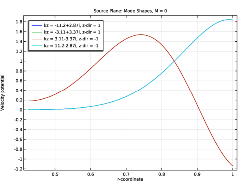
In the Settings window for 1D Plot Group, type Source Plane: Mode Shapes, M = 0 in the Label text field.
|
|
3
|
Locate the Data section. From the Dataset list, choose Study 2 - Source Plane Modes/Parametric Solutions 1 (sol3).
|
|
4
|
|
5
|
|
6
|
|
1
|
|
2
|
|
3
|
|
4
|
|
5
|
|
6
|
|
7
|
|
8
|
|
9
|
|
10
|
|
1
|
|
2
|
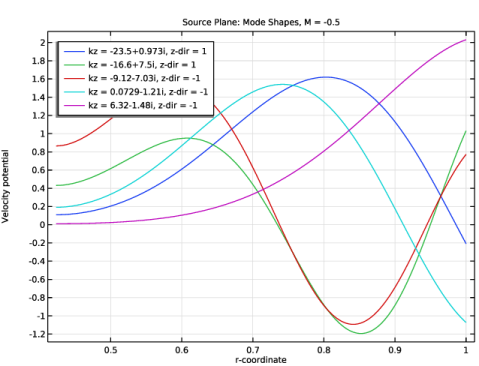
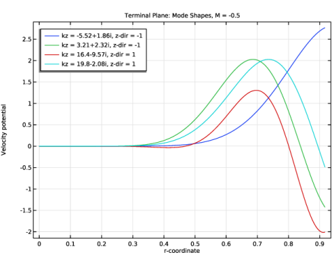
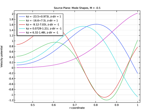
In the Settings window for 1D Plot Group, type Source Plane: Mode Shapes, M = -0.5 in the Label text field.
|
|
3
|
|
4
|
|
1
|
|
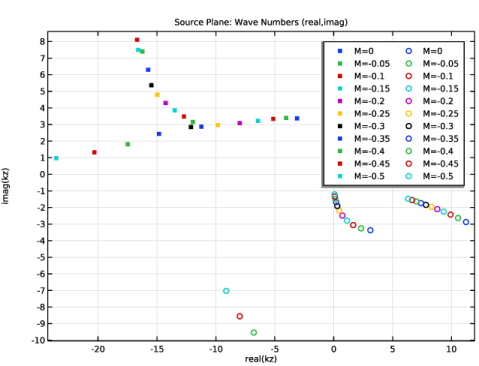
2
|
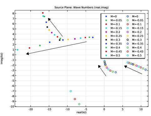
In the Settings window for 1D Plot Group, type Source Plane: Wave Numbers (real,imag) in the Label text field.
|
|
3
|
Locate the Data section. From the Dataset list, choose Study 2 - Source Plane Modes/Parametric Solutions 1 (sol3).
|
|
4
|
|
5
|
Locate the Plot Settings section.
|
|
6
|
|
7
|
|
8
|
|
1
|
|
2
|
|
4
|
|
5
|
|
6
|
|
7
|
Click to expand the Coloring and Style section. Find the Line style subsection. From the Line list, choose None.
|
|
8
|
|
1
|
|
2
|
|
3
|
|
1
|
In the Model Builder window, under Results > Source Plane: Wave Numbers (real,imag) right-click Global 1 and choose Duplicate.
|
|
2
|
|
3
|
|
4
|
|
1
|
|
2
|
|
3
|
|
4
|
|
1
|
|
2
|
Go to the Add Study window.
|
|
3
|
Find the Physics interfaces in study subsection. In the table, clear the Solve checkboxes for Compressible Potential Flow (cpf), Linearized Potential Flow, Boundary Mode (lpfbm), and Linearized Potential Flow, Frequency Domain (lpff).
|
|
4
|
Find the Studies subsection. In the Select Study tree, select Preset Studies for Selected Physics Interfaces > Mode Analysis.
|
|
5
|
Click the Add Study button in the window toolbar.
|
|
1
|
|
2
|
|
3
|
Click
|
|
1
|
|
2
|
|
3
|
|
4
|
|
5
|
|
6
|
|
7
|
Find the Rectangle search region subsection. In the Smallest real part (Out-of-plane wave number) text field, type -1.1*k0max_abs.
|
|
8
|
|
9
|
|
10
|
|
11
|
Click to expand the Values of Dependent Variables section. Find the Values of variables not solved for subsection. From the Settings list, choose User controlled.
|
|
12
|
|
13
|
|
14
|
|
15
|
|
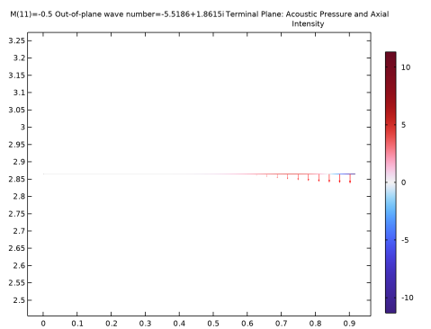
1
|
In the Settings window for 2D Plot Group, type Terminal Plane: Acoustic Pressure and Axial Intensity in the Label text field.
|
|
2
|
|
3
|
|
4
|
Select the Apply to dataset edges checkbox.
|
|
5
|
|
1
|
|
2
|
In the Settings window for Arrow Line, click Replace Expression in the upper-right corner of the Expression section. From the menu, choose Component 1 (comp1) > Linearized Potential Flow, Boundary Mode 2 > Intensity > lpfbm2.Ir,lpfbm2.Iz - Intensity.
|
|
3
|
|
4
|
|
5
|
|
1
|
|
2
|
|
3
|
|
1
|
|
2
|
|
3
|
|
1
|
|
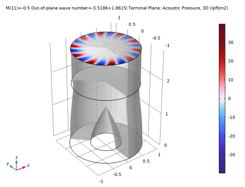
2
|
In the Settings window for 3D Plot Group, type Terminal Plane: Acoustic Pressure, 3D (lpfbm2) in the Label text field.
|
|
3
|
|
1
|
|
2
|
|
3
|
|
4
|
|
5
|
|
6
|
|
1
|
|
2
|
Click in the Graphics window and then press Ctrl+A to select both domains.
|
|
3
|
|
4
|
Clear the Evaluate the start cap checkbox.
|
|
5
|
Clear the Evaluate the end cap checkbox.
|
|
1
|
|
2
|
|
3
|
|
1
|
In the Model Builder window, under Results > Terminal Plane: Acoustic Pressure, 3D (lpfbm2) click Surface.
|
|
2
|
|
3
|
|
4
|
|
1
|
|
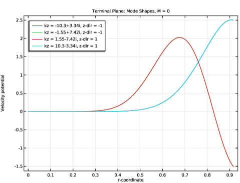
2
|
In the Settings window for 1D Plot Group, type Terminal Plane: Mode Shapes, M = 0 in the Label text field.
|
|
3
|
Locate the Data section. From the Dataset list, choose Study 3 - Terminal Plane Modes/Parametric Solutions 2 (sol16).
|
|
4
|
|
5
|
|
6
|
|
1
|
|
2
|
|
3
|
|
4
|
|
5
|
|
6
|
|
7
|
|
8
|
|
9
|
|
10
|
|
1
|
|
2
|
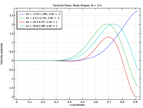
In the Settings window for 1D Plot Group, type Terminal Plane: Mode Shapes, M = -0.5 in the Label text field.
|
|
3
|
|
4
|
|
1
|
|
2
|
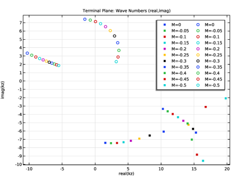
In the Settings window for 1D Plot Group, type Terminal Plane: Wave Numbers (real,imag) in the Label text field.
|
|
3
|
Locate the Data section. From the Dataset list, choose Study 3 - Terminal Plane Modes/Parametric Solutions 2 (sol16).
|
|
4
|
|
5
|
Locate the Plot Settings section.
|
|
6
|
|
7
|
|
8
|
|
1
|
|
2
|
|
4
|
|
5
|
|
6
|
|
7
|
Click to expand the Coloring and Style section. Find the Line style subsection. From the Line list, choose None.
|
|
8
|
|
1
|
|
2
|
|
3
|
|
1
|
In the Model Builder window, under Results > Terminal Plane: Wave Numbers (real,imag) right-click Global 1 and choose Duplicate.
|
|
2
|
|
3
|
|
4
|
|
1
|
|
2
|
|
3
|
|
4
|
|
1
|
In the Model Builder window, under Component 1 (comp1) click Linearized Potential Flow, Frequency Domain (lpff).
|
|
2
|
In the Settings window for Linearized Potential Flow, Frequency Domain, locate the Linearized Potential Flow Equation Settings section.
|
|
3
|
|
4
|
Locate the Global Port Settings section. From the Mode shape normalization list, choose Power normalization.
|
|
1
|
|
3
|
|
4
|
|
1
|
In the Model Builder window, right-click Linearized Potential Flow, Frequency Domain (lpff) and choose Node Group.
|
|
2
|
|
1
|
|
2
|
|
3
|
|
4
|
Locate the Port Outgoing Mode Settings section. In the ϕnout text field, type withsol('sol3',phi_sp,setval(M,-0.5),setind(lambda,5)).
|
|
5
|
|
6
|
Locate the Port Incident Mode Settings section. From the Incident wave excitation at this port list, choose On.
|
|
7
|
|
8
|
|
9
|
|
10
|
|
1
|
|
2
|
|
3
|
|
4
|
Locate the Port Outgoing Mode Settings section. In the ϕnout text field, type withsol('sol3',phi_sp,setval(M,-0.5),setind(lambda,4)).
|
|
5
|
|
1
|
|
2
|
|
1
|
|
2
|
|
3
|
|
4
|
Locate the Port Outgoing Mode Settings section. In the ϕnout text field, type withsol('sol16',phi_tp,setval(M,-0.5),setind(lambda,3)).
|
|
5
|
|
1
|
|
2
|
|
3
|
|
4
|
Locate the Port Outgoing Mode Settings section. In the ϕnout text field, type withsol('sol16',phi_tp,setval(M,-0.5),setind(lambda,4)).
|
|
5
|
|
1
|
|
2
|
Go to the Add Study window.
|
|
3
|
Find the Physics interfaces in study subsection. In the table, clear the Solve checkboxes for Compressible Potential Flow (cpf), Linearized Potential Flow, Boundary Mode (lpfbm), and Linearized Potential Flow, Boundary Mode 2 (lpfbm2).
|
|
4
|
|
5
|
Click the Add Study button in the window toolbar.
|
|
1
|
In the Model Builder window, under Study 4 - Frequency Domain (M = -0.5, lined) click Step 1: Frequency Domain.
|
|
2
|
|
3
|
|
4
|
Click to expand the Values of Dependent Variables section. Find the Values of variables not solved for subsection. From the Settings list, choose User controlled.
|
|
5
|
|
6
|
|
7
|
|
8
|
|
9
|
|
10
|
Clear the Generate default plots checkbox.
|
|
11
|
|
1
|
|
2
|
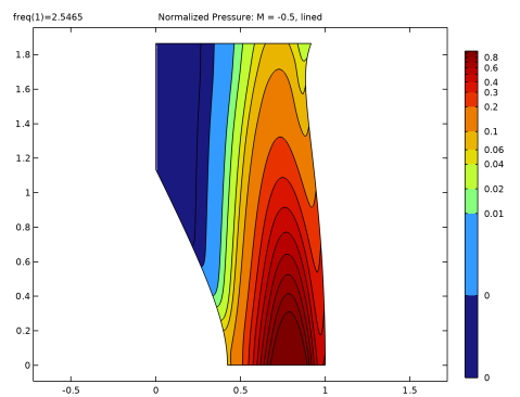
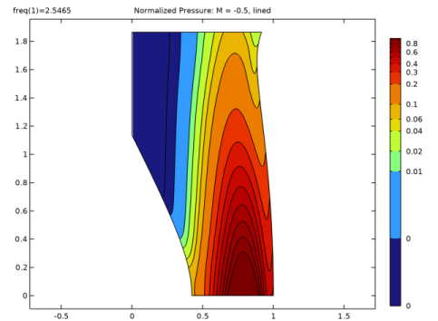
In the Settings window for 2D Plot Group, type Normalized Pressure: M = -0.5, lined in the Label text field.
|
|
3
|
Locate the Data section. From the Dataset list, choose Study 4 - Frequency Domain (M = -0.5, lined)/Solution 28 (sol28).
|
|
4
|
|
6
|
Select the Apply to dataset edges checkbox.
|
|
7
|
|
1
|
|
2
|
|
3
|
|
4
|
|
5
|
In the Levels text field, type 0.0001 0.001 0.01 0.02 0.04 0.06 0.1 0.2 0.3 0.4 0.5 0.6 0.7 0.8 0.9.
|
|
6
|
|
7
|
|
8
|
|
1
|
|
2
|
|
3
|
|
4
|
|
5
|
|
6
|
Clear the Color legend checkbox.
|
|
1
|
|
2
|
|
3
|
|
1
|
|
2
|
|
3
|
Locate the Data section. From the Dataset list, choose Study 4 - Frequency Domain (M = -0.5, lined)/Solution 28 (sol28).
|
|
1
|
|
2
|
|
3
|
|
1
|
|
2
|
|
3
|
|
5
|
Select the Apply to dataset edges checkbox.
|
|
1
|
|
2
|
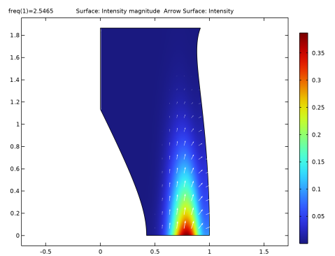
In the Settings window for Arrow Surface, click Replace Expression in the upper-right corner of the Expression section. From the menu, choose Component 1 (comp1) > Linearized Potential Flow, Frequency Domain > Intensity > lpff.Ir,lpff.Iz - Intensity.
|
|
3
|
|
4
|
|
5
|
|
6
|
|
1
|
|
2
|
In the Settings window for Evaluation Group, type Evaluation Group: Attenuation in the Label text field.
|
|
3
|
|
1
|
|
2
|
|
3
|
|
4
|
Locate the Expressions section. In the table, enter the following settings:
|
|
5
|