|
|
|

|
•
|
Sound hard — the normal component of the acoustic particle velocity vanishes at the boundary.
|
|
•
|
Impedance — the normal component of the acoustic particle velocity is related to the particle displacement through the equation
|
|
•
|
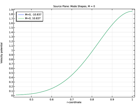
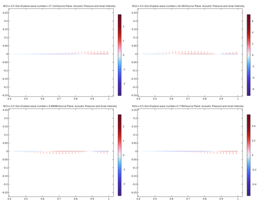
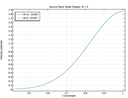
At the source plane in the no-flow case (M = 0), the outgoing mode has the wave number kn = 10.8. This is the second eigenvalue in solution list and thus as index 2 (necessary for referencing at the port). The incident mode (the source) has wave number kn = −10.8 (index 1).
|
|
•
|
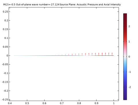
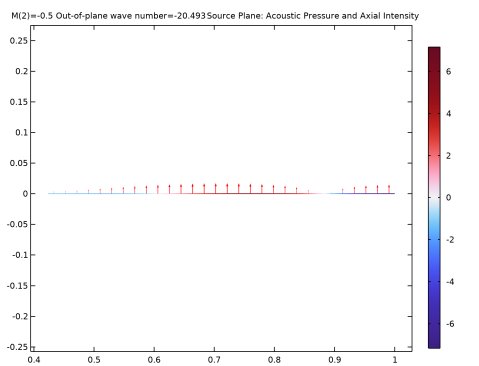
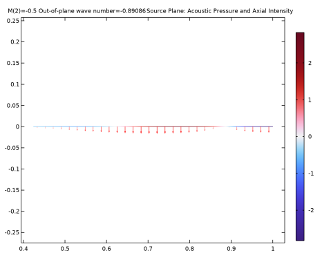
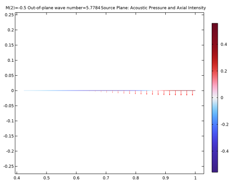
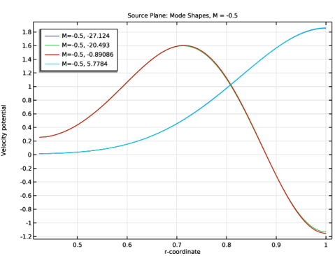
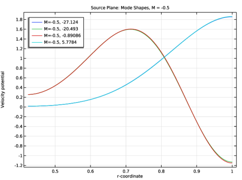
At the source plane in the flow case (M = −0.5), the outgoing modes have wave numbers are kn = −0.9 (index 3) and kn = 5.8 (index 4). The first incident radial mode (the source) has wave number kn = −27.1 (index 1). In the port condition it is advantageous for clarity (but not necessary) that modes corresponding to the same mode shape should be defined together. This means that the first radial modes (index 1 and 4) are referenced in one port, and the second outgoing radial mode (index 3) is referenced in the second port (where no source is added).
 |
|
•
|
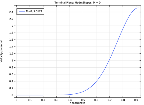
At the terminal plane in the no-flow case (M = 0), the outgoing mode has the wave number kn = 9.6. This is the first and only eigenvalue in solution list and has solution index 1 (necessary for referencing at the port). No incident mode is necessary as no source is defined here.
|
|
•
|
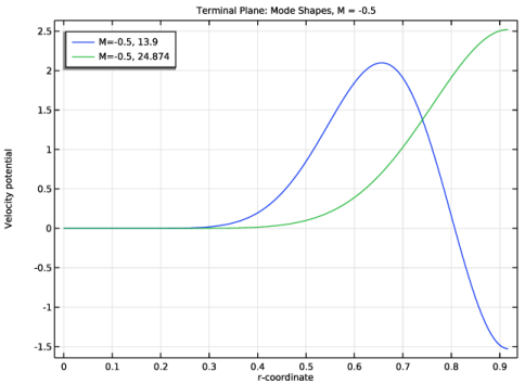
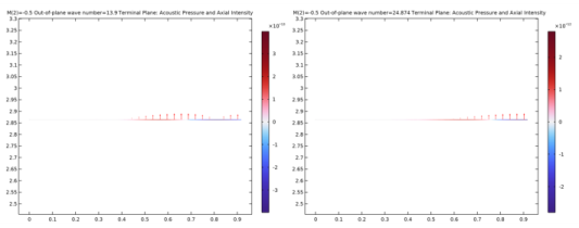
At the terminal plane in the flow case (M = −0.5), the outgoing modes have wave numbers kn = 13.9 (index 1) and kn = 24.9 (index 2). No incident mode is necessary as no source is defined here.
|
|
•
|
Compressible Potential Flow (cpf) — for modeling the background mean-flow velocity field as a potential flow (a lossless and irrotational flow).
|
|
•
|
Linearized Potential Flow, Boundary Mode (lpfbm) — for calculating the boundary eigenmode to be used by the port boundary conditions, defining outgoing and incident (the source) propagating acoustic field.
|
|
•
|
Linearized Potential Flow, Frequency Domain (lpff) — for modeling the time-harmonic acoustic field in the duct for the various excitation and flow condition.
|
|
1
|
|
2
|
|
3
|
Click Add.
|
|
4
|
In the Select Physics tree, select Acoustics > Aeroacoustics > Linearized Potential Flow, Boundary Mode (lpfbm).
|
|
5
|
Click Add.
|
|
6
|
|
7
|
In the Select Physics tree, select Acoustics > Aeroacoustics > Linearized Potential Flow, Boundary Mode (lpfbm).
|
|
8
|
Click Add.
|
|
9
|
|
10
|
In the Select Physics tree, select Acoustics > Aeroacoustics > Linearized Potential Flow, Frequency Domain (lpff).
|
|
11
|
Click Add.
|
|
12
|
Click
|
|
13
|
|
14
|
Click
|
|
1
|
In the Model Builder window, click the root node.
|
|
2
|
|
3
|
|
1
|
|
2
|
|
3
|
Click
|
|
4
|
Browse to the model’s Application Libraries folder and double-click the file flow_duct_boundary_mode_parameters.txt.
|
|
1
|
|
2
|
|
3
|
|
4
|
|
1
|
|
2
|
|
3
|
|
4
|
|
5
|
|
1
|
|
2
|
|
3
|
|
4
|
|
5
|
|
1
|
|
2
|
|
1
|
|
2
|
|
3
|
|
4
|
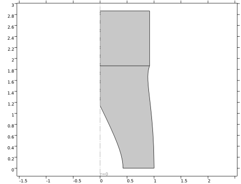
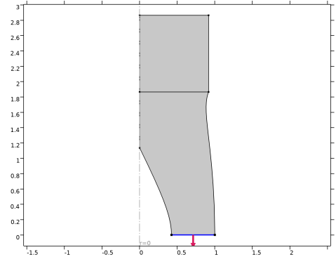
On the object uni1, select Point 5 only.
|
|
5
|
|
6
|
On the object pc1, select Point 1 only.
|
|
1
|
|
2
|
On the object uni1, select Point 4 only.
|
|
3
|
|
4
|
|
5
|
On the object pc1, select Point 2 only.
|
|
6
|
|
1
|
|
2
|
On the object uni1, select Boundaries 1 and 3 only.
|
|
3
|
|
1
|
|
2
|
Click in the Graphics window and then press Ctrl+D to clear all objects.
|
|
3
|
|
1
|
|
2
|
|
3
|
|
4
|
|
1
|
|
2
|
|
3
|
|
1
|
In the Model Builder window, under Component 1 (comp1) right-click Definitions and choose Variables.
|
|
2
|
|
3
|
|
5
|
Locate the Variables section. In the table, enter the following settings:
|
|
1
|
|
2
|
|
3
|
|
1
|
|
2
|
|
3
|
|
1
|
|
2
|
|
3
|
|
1
|
|
1
|
|
2
|
|
3
|
|
4
|
|
1
|
|
2
|
|
3
|
|
4
|
|
1
|
|
2
|
|
3
|
|
4
|
|
5
|
|
1
|
In the Model Builder window, under Component 1 (comp1) > Compressible Potential Flow (cpf) click Compressible Potential Flow Model 1.
|
|
2
|
In the Settings window for Compressible Potential Flow Model, locate the Compressible Potential Flow Model section.
|
|
3
|
|
1
|
|
2
|
|
3
|
|
1
|
|
2
|
|
3
|
|
1
|
In the Model Builder window, under Component 1 (comp1) click Linearized Potential Flow, Boundary Mode (lpfbm).
|
|
2
|
In the Settings window for Linearized Potential Flow, Boundary Mode, locate the Boundary Selection section.
|
|
3
|
|
4
|
|
1
|
In the Model Builder window, under Component 1 (comp1) > Linearized Potential Flow, Boundary Mode (lpfbm) click Linearized Potential Flow Model 1.
|
|
2
|
|
3
|
|
4
|
|
5
|
|
1
|
In the Model Builder window, under Component 1 (comp1) click Linearized Potential Flow, Boundary Mode 2 (lpfbm2).
|
|
2
|
In the Settings window for Linearized Potential Flow, Boundary Mode, locate the Boundary Selection section.
|
|
3
|
|
4
|
|
1
|
In the Model Builder window, under Component 1 (comp1) > Linearized Potential Flow, Boundary Mode 2 (lpfbm2) click Linearized Potential Flow Model 1.
|
|
2
|
|
3
|
|
4
|
|
5
|
|
1
|
|
2
|
|
3
|
|
1
|
|
2
|
|
3
|
Click the Custom button.
|
|
4
|
|
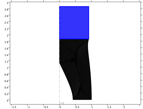
6
|
Locate the Element Size Parameters section.
|
|
7
|
|
1
|
|
2
|
|
3
|
Click the Custom button.
|
|
4
|
|
5
|
|
1
|
|
2
|
|
1
|
|
2
|
|
1
|
|
2
|
|
3
|
Click
|
|
5
|
|
1
|
|
2
|
|
3
|
|
4
|
|
1
|
|
2
|
|
3
|
|
4
|
|
5
|
|
1
|
|
2
|
|
3
|
|
4
|
|
5
|
|
6
|
|
1
|
|
2
|
|
3
|
|
4
|
|
5
|
|
6
|
|
7
|
|
8
|
|
9
|
|
1
|
|
2
|
|
3
|
|
4
|
|
5
|
|
6
|
|
7
|
|
8
|
|
9
|
|
1
|
|
2
|
Go to the Add Study window.
|
|
3
|
Find the Physics interfaces in study subsection. In the table, clear the Solve checkboxes for Compressible Potential Flow (cpf), Linearized Potential Flow, Boundary Mode 2 (lpfbm2), and Linearized Potential Flow, Frequency Domain (lpff).
|
|
4
|
Find the Studies subsection. In the Select Study tree, select Preset Studies for Selected Physics Interfaces > Mode Analysis.
|
|
5
|
Click the Add Study button in the window toolbar.
|
|
1
|
|
2
|
|
3
|
Click
|
|
1
|
|
2
|
|
3
|
|
4
|
|
5
|
|
6
|
|
7
|
Find the Rectangle search region subsection. In the Smallest real part (Out-of-plane wave number) text field, type -1.1*k0max_abs.
|
|
8
|
|
9
|
|
10
|
|
11
|
Click to expand the Values of Dependent Variables section. Find the Values of variables not solved for subsection. From the Settings list, choose User controlled.
|
|
12
|
|
13
|
|
14
|
|
15
|
|
1
|
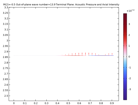
In the Settings window for 2D Plot Group, type Source Plane: Acoustic Pressure and Axial Intensity in the Label text field.
|
|
2
|
|
3
|
|
4
|
Select the Apply to dataset edges checkbox.
|
|
5
|
|
1
|
|
2
|
In the Settings window for Arrow Line, click Replace Expression in the upper-right corner of the Expression section. From the menu, choose Component 1 (comp1) > Linearized Potential Flow, Boundary Mode > Intensity > lpfbm.Ir,lpfbm.Iz - Intensity.
|
|
3
|
|
4
|
|
5
|
|
1
|
|
2
|
|
3
|
|
4
|
|
5
|
|
6
|
|
7
|
|
8
|
|
9
|
|
10
|
|
1
|
|
2
|
|
3
|
|
1
|
|
2
|
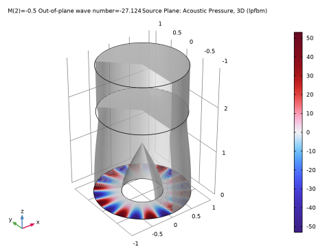
In the Settings window for 3D Plot Group, type Source Plane: Acoustic Pressure, 3D (lpfbm) in the Label text field.
|
|
3
|
|
1
|
|
2
|
|
3
|
|
4
|
|
5
|
|
6
|
|
1
|
|
2
|
Click in the Graphics window and then press Ctrl+A to select both domains.
|
|
3
|
|
4
|
Clear the Evaluate the start cap checkbox.
|
|
5
|
Clear the Evaluate the end cap checkbox.
|
|
1
|
|
2
|
|
3
|
|
1
|
In the Model Builder window, under Results > Source Plane: Acoustic Pressure, 3D (lpfbm) click Surface.
|
|
2
|
|
3
|
|
4
|
|
1
|
|
2
|
In the Settings window for 1D Plot Group, type Source Plane: Mode Shapes, M = 0 in the Label text field.
|
|
3
|
Locate the Data section. From the Dataset list, choose Study 2 - Source Plane Modes/Parametric Solutions 1 (sol3).
|
|
4
|
|
5
|
|
6
|
|
1
|
|
2
|
|
3
|
|
4
|
|
5
|
|
6
|
|
7
|
|
8
|
|
1
|
|
2
|
In the Settings window for 1D Plot Group, type Source Plane: Mode Shapes, M = -0.5 in the Label text field.
|
|
3
|
|
4
|
|
1
|
|
2
|
Go to the Add Study window.
|
|
3
|
Find the Physics interfaces in study subsection. In the table, clear the Solve checkboxes for Compressible Potential Flow (cpf), Linearized Potential Flow, Boundary Mode (lpfbm), and Linearized Potential Flow, Frequency Domain (lpff).
|
|
4
|
Find the Studies subsection. In the Select Study tree, select Preset Studies for Selected Physics Interfaces > Mode Analysis.
|
|
5
|
Click the Add Study button in the window toolbar.
|
|
1
|
|
2
|
|
3
|
Click
|
|
1
|
|
2
|
|
3
|
|
4
|
|
5
|
|
6
|
|
7
|
Find the Rectangle search region subsection. In the Smallest real part (Out-of-plane wave number) text field, type -1.1*k0max_abs.
|
|
8
|
|
9
|
|
10
|
|
11
|
Locate the Values of Dependent Variables section. Find the Values of variables not solved for subsection. From the Settings list, choose User controlled.
|
|
12
|
|
13
|
|
14
|
|
15
|
Click to expand the Filtering and Sorting section. Find the Filtering subsection. In the table, enter the following settings:
|
|
16
|
|
1
|
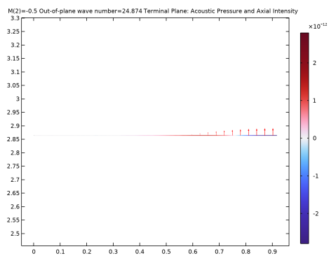
In the Settings window for 2D Plot Group, type Terminal Plane: Acoustic Pressure and Axial Intensity in the Label text field.
|
|
2
|
|
3
|
|
4
|
Select the Apply to dataset edges checkbox.
|
|
5
|
|
1
|
|
2
|
In the Settings window for Arrow Line, click Replace Expression in the upper-right corner of the Expression section. From the menu, choose Component 1 (comp1) > Linearized Potential Flow, Boundary Mode 2 > Intensity > lpfbm2.Ir,lpfbm2.Iz - Intensity.
|
|
3
|
|
4
|
|
5
|
|
1
|
|
2
|
|
3
|
|
4
|
|
5
|
|
6
|
|
1
|
|
2
|
|
3
|
|
1
|
|
2
|
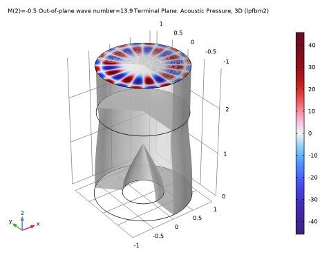
In the Settings window for 3D Plot Group, type Terminal Plane: Acoustic Pressure, 3D (lpfbm2) in the Label text field.
|
|
3
|
|
1
|
|
2
|
|
3
|
|
4
|
|
5
|
|
6
|
|
1
|
|
2
|
Click in the Graphics window and then press Ctrl+A to select both domains.
|
|
3
|
|
4
|
Clear the Evaluate the start cap checkbox.
|
|
5
|
Clear the Evaluate the end cap checkbox.
|
|
1
|
|
2
|
|
3
|
|
1
|
In the Model Builder window, under Results > Terminal Plane: Acoustic Pressure, 3D (lpfbm2) click Surface.
|
|
2
|
|
3
|
|
4
|
|
1
|
|
2
|
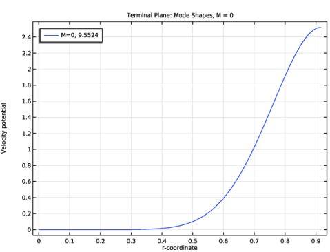
In the Settings window for 1D Plot Group, type Terminal Plane: Mode Shapes, M = 0 in the Label text field.
|
|
3
|
Locate the Data section. From the Dataset list, choose Study 3 - Terminal Plane Modes/Parametric Solutions 2 (sol7).
|
|
4
|
|
5
|
|
6
|
|
1
|
|
2
|
|
3
|
|
4
|
|
5
|
|
6
|
|
7
|
|
8
|
|
1
|
|
2
|
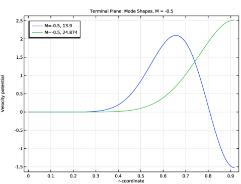
In the Settings window for 1D Plot Group, type Terminal Plane: Mode Shapes, M = -0.5 in the Label text field.
|
|
3
|
|
4
|
|
1
|
In the Model Builder window, under Component 1 (comp1) click Linearized Potential Flow, Frequency Domain (lpff).
|
|
2
|
In the Settings window for Linearized Potential Flow, Frequency Domain, locate the Linearized Potential Flow Equation Settings section.
|
|
3
|
|
4
|
Locate the Global Port Settings section. From the Mode shape normalization list, choose Power normalization.
|
|
1
|
|
3
|
|
4
|
|
1
|
In the Model Builder window, right-click Linearized Potential Flow, Frequency Domain (lpff) and choose Node Group.
|
|
2
|
|
1
|
|
2
|
|
3
|
|
4
|
|
5
|
Locate the Port Outgoing Mode Settings section. In the ϕnout text field, type withsol('sol3',phi_sp,setval(M,0),setind(lambda,2)).
|
|
6
|
|
7
|
Locate the Port Incident Mode Settings section. From the Incident wave excitation at this port list, choose On.
|
|
8
|
|
9
|
|
10
|
|
11
|
|
1
|
|
2
|
|
3
|
|
4
|
|
5
|
Locate the Port Outgoing Mode Settings section. In the ϕnout text field, type withsol('sol3',phi_sp,setval(M,-0.5),setind(lambda,4)).
|
|
6
|
|
7
|
Locate the Port Incident Mode Settings section. From the Incident wave excitation at this port list, choose On.
|
|
8
|
|
9
|
|
10
|
|
11
|
|
1
|
|
2
|
|
3
|
|
4
|
|
5
|
Locate the Port Outgoing Mode Settings section. In the ϕnout text field, type withsol('sol3',phi_sp,setval(M,-0.5),setind(lambda,3)).
|
|
6
|
|
1
|
|
2
|
|
1
|
|
2
|
|
3
|
|
4
|
Locate the Port Outgoing Mode Settings section. In the ϕnout text field, type withsol('sol7',phi_tp,setval(M,0),setind(lambda,1)).
|
|
5
|
|
1
|
|
2
|
|
3
|
|
4
|
|
5
|
Locate the Port Outgoing Mode Settings section. In the ϕnout text field, type withsol('sol7',phi_tp,setval(M,-0.5),setind(lambda,1)).
|
|
6
|
|
1
|
|
2
|
|
3
|
|
4
|
|
5
|
Locate the Port Outgoing Mode Settings section. In the ϕnout text field, type withsol('sol7',phi_tp,setval(M,-0.5),setind(lambda,2)).
|
|
6
|
|
1
|
|
2
|
Go to the Add Study window.
|
|
3
|
Find the Physics interfaces in study subsection. In the table, clear the Solve checkboxes for Compressible Potential Flow (cpf), Linearized Potential Flow, Boundary Mode (lpfbm), and Linearized Potential Flow, Boundary Mode 2 (lpfbm2).
|
|
4
|
|
5
|
Click the Add Study button in the window toolbar.
|
|
1
|
In the Model Builder window, under Study 4 - Frequency Domain (M = 0, lined) click Step 1: Frequency Domain.
|
|
2
|
|
3
|
|
4
|
Locate the Physics and Variables Selection section. Select the Modify model configuration for study step checkbox.
|
|
5
|
In the tree, select Component 1 (comp1) > Linearized Potential Flow, Frequency Domain (lpff) > Source Plane > Port 2 (for M = -0.5), Component 1 (comp1) > Linearized Potential Flow, Frequency Domain (lpff) > Source Plane > Port 3 (for M = -0.5), Component 1 (comp1) > Linearized Potential Flow, Frequency Domain (lpff) > Terminal Plane > Port 5 (for M = -0.5), and Component 1 (comp1) > Linearized Potential Flow, Frequency Domain (lpff) > Terminal Plane > Port 6 (for M = -0.5).
|
|
6
|
Click
|
|
7
|
Click to expand the Values of Dependent Variables section. Find the Values of variables not solved for subsection. From the Settings list, choose User controlled.
|
|
8
|
|
9
|
|
10
|
|
11
|
|
12
|
|
13
|
Clear the Generate default plots checkbox.
|
|
14
|
|
1
|
|
2
|
Go to the Add Study window.
|
|
3
|
Find the Physics interfaces in study subsection. In the table, clear the Solve checkboxes for Compressible Potential Flow (cpf), Linearized Potential Flow, Boundary Mode (lpfbm), and Linearized Potential Flow, Boundary Mode 2 (lpfbm2).
|
|
4
|
|
5
|
Click the Add Study button in the window toolbar.
|
|
1
|
In the Model Builder window, under Study 5 - Frequency Domain (M = 0, hard) click Step 1: Frequency Domain.
|
|
2
|
|
3
|
|
4
|
Locate the Physics and Variables Selection section. Select the Modify model configuration for study step checkbox.
|
|
5
|
In the tree, select Component 1 (comp1) > Linearized Potential Flow, Frequency Domain (lpff) > Impedance 1, Component 1 (comp1) > Linearized Potential Flow, Frequency Domain (lpff) > Source Plane > Port 2 (for M = -0.5), Component 1 (comp1) > Linearized Potential Flow, Frequency Domain (lpff) > Source Plane > Port 3 (for M = -0.5), Component 1 (comp1) > Linearized Potential Flow, Frequency Domain (lpff) > Terminal Plane > Port 5 (for M = -0.5), and Component 1 (comp1) > Linearized Potential Flow, Frequency Domain (lpff) > Terminal Plane > Port 6 (for M = -0.5).
|
|
6
|
Click
|
|
7
|
Locate the Values of Dependent Variables section. Find the Values of variables not solved for subsection. From the Settings list, choose User controlled.
|
|
8
|
|
9
|
|
10
|
|
11
|
|
12
|
|
13
|
Clear the Generate default plots checkbox.
|
|
14
|
|
1
|
|
2
|
Go to the Add Study window.
|
|
3
|
Find the Physics interfaces in study subsection. In the table, clear the Solve checkboxes for Compressible Potential Flow (cpf), Linearized Potential Flow, Boundary Mode (lpfbm), and Linearized Potential Flow, Boundary Mode 2 (lpfbm2).
|
|
4
|
|
5
|
Click the Add Study button in the window toolbar.
|
|
1
|
In the Model Builder window, under Study 6 - Frequency Domain (M = -0.5, lined) click Step 1: Frequency Domain.
|
|
2
|
|
3
|
|
4
|
Locate the Physics and Variables Selection section. Select the Modify model configuration for study step checkbox.
|
|
5
|
In the tree, select Component 1 (comp1) > Linearized Potential Flow, Frequency Domain (lpff) > Source Plane > Port 1 (for M = 0) and Component 1 (comp1) > Linearized Potential Flow, Frequency Domain (lpff) > Terminal Plane > Port 4 (for M = 0).
|
|
6
|
Click
|
|
7
|
Locate the Values of Dependent Variables section. Find the Values of variables not solved for subsection. From the Settings list, choose User controlled.
|
|
8
|
|
9
|
|
10
|
|
11
|
|
12
|
|
13
|
Clear the Generate default plots checkbox.
|
|
14
|
|
1
|
|
2
|
Go to the Add Study window.
|
|
3
|
Find the Physics interfaces in study subsection. In the table, clear the Solve checkboxes for Compressible Potential Flow (cpf), Linearized Potential Flow, Boundary Mode (lpfbm), and Linearized Potential Flow, Boundary Mode 2 (lpfbm2).
|
|
4
|
|
5
|
Click the Add Study button in the window toolbar.
|
|
1
|
In the Model Builder window, under Study 7 - Frequency Domain (M = -0.5, hard) click Step 1: Frequency Domain.
|
|
2
|
|
3
|
|
4
|
Locate the Physics and Variables Selection section. Select the Modify model configuration for study step checkbox.
|
|
5
|
In the tree, select Component 1 (comp1) > Linearized Potential Flow, Frequency Domain (lpff) > Impedance 1, Component 1 (comp1) > Linearized Potential Flow, Frequency Domain (lpff) > Source Plane > Port 1 (for M = 0), and Component 1 (comp1) > Linearized Potential Flow, Frequency Domain (lpff) > Terminal Plane > Port 4 (for M = 0).
|
|
6
|
Click
|
|
7
|
Locate the Values of Dependent Variables section. Find the Values of variables not solved for subsection. From the Settings list, choose User controlled.
|
|
8
|
|
9
|
|
10
|
|
11
|
|
12
|
|
13
|
Clear the Generate default plots checkbox.
|
|
14
|
|
1
|
|
2
|
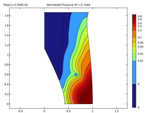
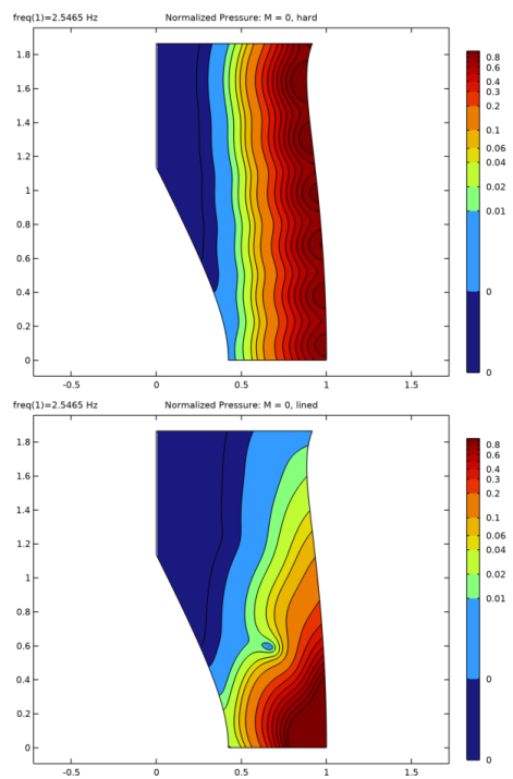
In the Settings window for 2D Plot Group, type Normalized Pressure: M = 0, lined in the Label text field.
|
|
3
|
Locate the Data section. From the Dataset list, choose Study 4 - Frequency Domain (M = 0, lined)/Solution 10 (sol10).
|
|
4
|
|
6
|
Select the Apply to dataset edges checkbox.
|
|
7
|
|
1
|
|
2
|
|
3
|
|
4
|
|
5
|
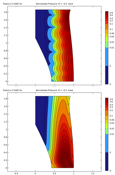
In the Levels text field, type 0.0001 0.001 0.01 0.02 0.04 0.06 0.1 0.2 0.3 0.4 0.5 0.6 0.7 0.8 0.9.
|
|
6
|
|
7
|
|
8
|
|
1
|
|
2
|
|
3
|
|
4
|
|
5
|
|
6
|
Clear the Color legend checkbox.
|
|
1
|
|
2
|
|
3
|
|
1
|
|
2
|
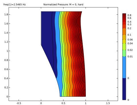
In the Settings window for 2D Plot Group, type Normalized Pressure: M = 0, hard in the Label text field.
|
|
3
|
Locate the Data section. From the Dataset list, choose Study 5 - Frequency Domain (M = 0, hard)/Solution 11 (sol11).
|
|
4
|
|
1
|
|
2
|
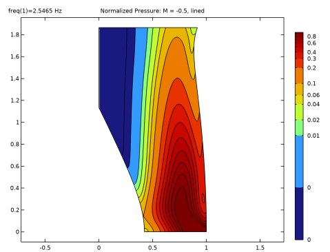
In the Settings window for 2D Plot Group, type Normalized Pressure: M = -0.5, lined in the Label text field.
|
|
3
|
Locate the Data section. From the Dataset list, choose Study 6 - Frequency Domain (M = -0.5, lined)/Solution 12 (sol12).
|
|
4
|
|
1
|
|
2
|
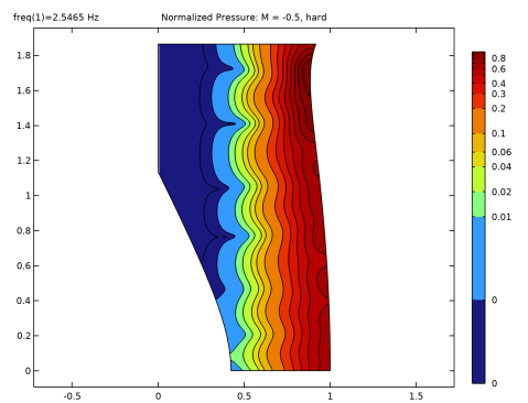
In the Settings window for 2D Plot Group, type Normalized Pressure: M = -0.5, hard in the Label text field.
|
|
3
|
Locate the Data section. From the Dataset list, choose Study 7 - Frequency Domain (M = -0.5, hard)/Solution 13 (sol13).
|
|
4
|
|
1
|
|
2
|
In the Settings window for Evaluation Group, type Evaluation Group: Attenuation in the Label text field.
|
|
3
|
|
1
|
|
2
|
|
3
|
|
4
|
Locate the Expressions section. In the table, enter the following settings:
|
|
1
|
In the Model Builder window, right-click Evaluation Group: Attenuation and choose Global Evaluation.
|
|
2
|
|
3
|
|
4
|
Locate the Expressions section. In the table, enter the following settings:
|
|
5
|
|
1
|
|
2
|
In the Settings window for Evaluation Group, type Source Plane: Mode Solution Index in the Label text field.
|
|
3
|
Locate the Data section. From the Dataset list, choose Study 2 - Source Plane Modes/Parametric Solutions 1 (sol3).
|
|
4
|
|
1
|
|
2
|
|
3
|
|
4
|
Locate the Expressions section. In the table, enter the following settings:
|
|
5
|
|
1
|
|
2
|
In the Settings window for Evaluation Group, type Terminal Plane: Mode Solution Index in the Label text field.
|
|
3
|
Locate the Data section. From the Dataset list, choose Study 3 - Terminal Plane Modes/Parametric Solutions 2 (sol7).
|
|
1
|
In the Model Builder window, expand the Terminal Plane: Mode Solution Index node, then click Global Evaluation 1.
|
|
2
|
|
4
|