|
|
|
|
•
|
Flow Duct — With Boundary Mode Analysis, where the hard walled port modes are computed using the boundary mode physics interface.
|
|
•
|
Flow Duct — Modes with Impedance Condition, where the mode computation includes the impedance conditions.
 |

|
•
|
Sound hard — the normal component of the acoustic particle velocity vanishes at the boundary.
|
|
•
|
Impedance — the normal component of the acoustic particle velocity is related to the particle displacement through the equation
|
|
•
|
Compressible Potential Flow (cpf) — for modeling the background mean-flow velocity field as a potential flow (a lossless and irrotational flow).
|
|
•
|
Linearized Potential Flow, Frequency Domain (lpff) — for modeling the time-harmonic acoustic field in the duct for the various excitation and flow condition. The Port condition is used at the source and terminal planes using the built-in Annular and Circular port type options.
|

|
1
|
|
2
|
|
3
|
Click Add.
|
|
4
|
In the Select Physics tree, select Acoustics > Aeroacoustics > Linearized Potential Flow, Frequency Domain (lpff).
|
|
5
|
Click Add.
|
|
6
|
Click
|
|
7
|
|
8
|
Click
|
|
1
|
In the Model Builder window, click the root node.
|
|
2
|
|
3
|
|
1
|
|
2
|
|
3
|
Click
|
|
4
|
Browse to the model’s Application Libraries folder and double-click the file flow_duct_parameters.txt.
|
|
1
|
|
2
|
|
3
|
|
4
|
|
1
|
|
2
|
|
3
|
|
4
|
|
5
|
|
1
|
|
2
|
|
3
|
|
4
|
|
5
|
|
1
|
|
2
|
|
1
|
|
2
|
|
3
|
|
4
|
On the object uni1, select Point 5 only.
|
|
5
|
|
6
|
On the object pc1, select Point 1 only.
|
|
1
|
|
2
|
On the object uni1, select Point 4 only.
|
|
3
|
|
4
|
|
5
|
On the object pc1, select Point 2 only.
|
|
6
|
|
1
|
|
2
|
On the object uni1, select Boundaries 1 and 3 only.
|
|
3
|
|
1
|
|
2
|
Click in the Graphics window and then press Ctrl+D to clear all objects.
|
|
3
|
|
1
|
|
2
|
|
3
|
|
4
|
|
1
|
|
2
|
|
3
|
|
1
|
In the Model Builder window, under Component 1 (comp1) right-click Definitions and choose Variables.
|
|
2
|
|
3
|
|
5
|
Locate the Variables section. In the table, enter the following settings:
|
|
1
|
|
2
|
|
3
|
|
1
|
|
2
|
|
3
|
|
1
|
|
2
|
|
3
|
|
1
|
|
1
|
|
2
|
|
3
|
|
4
|
|
1
|
|
2
|
|
3
|
|
4
|
|
5
|
|
1
|
In the Model Builder window, under Component 1 (comp1) > Compressible Potential Flow (cpf) click Compressible Potential Flow Model 1.
|
|
2
|
In the Settings window for Compressible Potential Flow Model, locate the Compressible Potential Flow Model section.
|
|
3
|
|
1
|
|
2
|
|
3
|
|
1
|
|
2
|
|
3
|
|
1
|
|
2
|
|
3
|
|
1
|
|
2
|
|
3
|
Click the Custom button.
|
|
4
|
|
6
|
Locate the Element Size Parameters section.
|
|
7
|
|
1
|
|
2
|
|
3
|
Click the Custom button.
|
|
4
|
|
5
|
|
1
|
|
2
|
|
1
|
|
2
|
|
1
|
|
2
|
|
3
|
Click
|
|
5
|
|
1
|
|
2
|
|
3
|
|
4
|
|
1
|
|
2
|
|
3
|
|
4
|
|
5
|
|
1
|
|
2
|
|
3
|
|
4
|
|
5
|
|
6
|
|
1
|
|
2
|
|
3
|
|
4
|
|
5
|
|
6
|
|
7
|
|
8
|
|
9
|
|
1
|
|
2
|
|
3
|
|
4
|
|
5
|
|
6
|
|
7
|
|
8
|
|
9
|
|
1
|
In the Model Builder window, under Component 1 (comp1) click Linearized Potential Flow, Frequency Domain (lpff).
|
|
2
|
In the Settings window for Linearized Potential Flow, Frequency Domain, locate the Linearized Potential Flow Equation Settings section.
|
|
3
|
|
4
|
Locate the Global Port Settings section. From the Mode shape normalization list, choose Power normalization.
|
|
1
|
|
3
|
|
4
|
|
1
|
In the Model Builder window, right-click Linearized Potential Flow, Frequency Domain (lpff) and choose Node Group.
|
|
2
|
|
1
|
|
2
|
|
3
|
|
4
|
|
5
|
Locate the Port Incident Mode Settings section. From the Incident wave excitation at this port list, choose On.
|
|
6
|
|
7
|
|
1
|
|
2
|
|
3
|
|
4
|
|
5
|
|
1
|
|
2
|
|
1
|
|
2
|
|
3
|
|
4
|
|
1
|
|
2
|
|
3
|
|
4
|
|
5
|
|
1
|
|
2
|
Go to the Add Study window.
|
|
3
|
Find the Physics interfaces in study subsection. In the table, clear the Solve checkbox for Compressible Potential Flow (cpf).
|
|
4
|
|
5
|
Click the Add Study button in the window toolbar.
|
|
1
|
In the Model Builder window, under Study 2 - Frequency Domain (M = 0, lined) click Step 1: Frequency Domain.
|
|
2
|
|
3
|
|
4
|
Click to expand the Values of Dependent Variables section. Find the Values of variables not solved for subsection. From the Settings list, choose User controlled.
|
|
5
|
|
6
|
|
7
|
|
8
|
|
9
|
|
10
|
Clear the Generate default plots checkbox.
|
|
11
|
|
1
|
|
2
|
Go to the Add Study window.
|
|
3
|
Find the Physics interfaces in study subsection. In the table, clear the Solve checkbox for Compressible Potential Flow (cpf).
|
|
4
|
|
5
|
Click the Add Study button in the window toolbar.
|
|
1
|
In the Model Builder window, under Study 3 - Frequency Domain (M = 0, hard) click Step 1: Frequency Domain.
|
|
2
|
|
3
|
|
4
|
Locate the Physics and Variables Selection section. Select the Modify model configuration for study step checkbox.
|
|
5
|
In the tree, select Component 1 (comp1) > Linearized Potential Flow, Frequency Domain (lpff) > Impedance 1.
|
|
6
|
Click
|
|
7
|
Click to expand the Values of Dependent Variables section. Find the Values of variables not solved for subsection. From the Settings list, choose User controlled.
|
|
8
|
|
9
|
|
10
|
|
11
|
|
12
|
|
13
|
Clear the Generate default plots checkbox.
|
|
14
|
|
1
|
|
2
|
Go to the Add Study window.
|
|
3
|
Find the Physics interfaces in study subsection. In the table, clear the Solve checkbox for Compressible Potential Flow (cpf).
|
|
4
|
|
5
|
Click the Add Study button in the window toolbar.
|
|
1
|
In the Model Builder window, under Study 4 - Frequency Domain (M = -0.5, lined) click Step 1: Frequency Domain.
|
|
2
|
|
3
|
|
4
|
Click to expand the Values of Dependent Variables section. Find the Values of variables not solved for subsection. From the Settings list, choose User controlled.
|
|
5
|
|
6
|
|
7
|
|
8
|
|
9
|
|
10
|
Clear the Generate default plots checkbox.
|
|
11
|
|
1
|
|
2
|
Go to the Add Study window.
|
|
3
|
Find the Physics interfaces in study subsection. In the table, clear the Solve checkbox for Compressible Potential Flow (cpf).
|
|
4
|
|
5
|
Click the Add Study button in the window toolbar.
|
|
1
|
In the Model Builder window, under Study 5 - Frequency Domain (M = -0.5, hard) click Step 1: Frequency Domain.
|
|
2
|
|
3
|
|
4
|
Locate the Physics and Variables Selection section. Select the Modify model configuration for study step checkbox.
|
|
5
|
In the tree, select Component 1 (comp1) > Linearized Potential Flow, Frequency Domain (lpff) > Impedance 1.
|
|
6
|
Click
|
|
7
|
Click to expand the Values of Dependent Variables section. Find the Values of variables not solved for subsection. From the Settings list, choose User controlled.
|
|
8
|
|
9
|
|
10
|
|
11
|
|
12
|
|
13
|
Clear the Generate default plots checkbox.
|
|
14
|
|
1
|
|
2
|
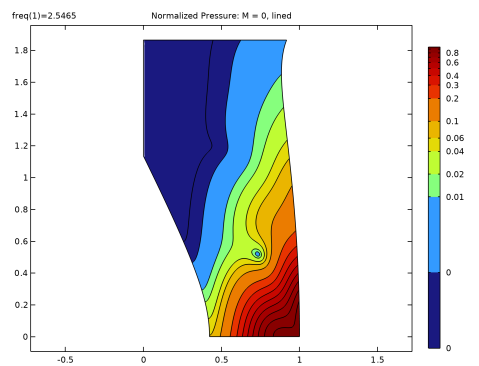
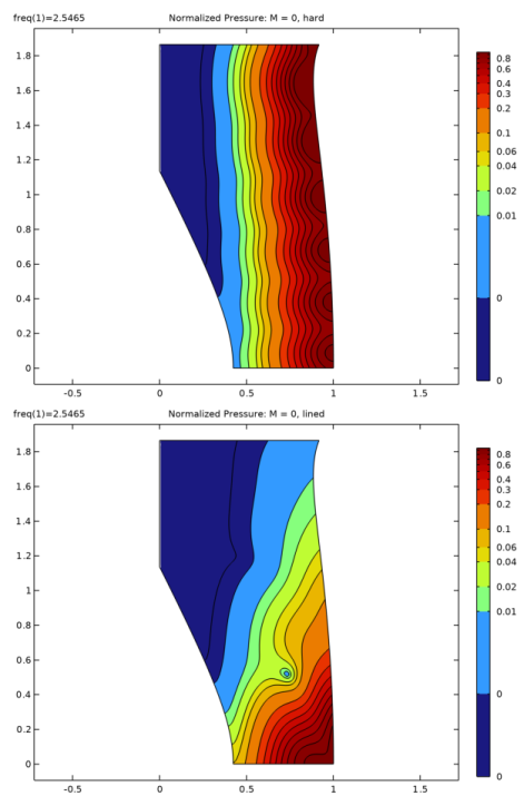
In the Settings window for 2D Plot Group, type Normalized Pressure: M = 0, lined in the Label text field.
|
|
3
|
Locate the Data section. From the Dataset list, choose Study 2 - Frequency Domain (M = 0, lined)/Solution 2 (sol2).
|
|
4
|
|
6
|
Select the Apply to dataset edges checkbox.
|
|
7
|
|
1
|
|
2
|
|
3
|
|
4
|
|
5
|
In the Levels text field, type 0.0001 0.001 0.01 0.02 0.04 0.06 0.1 0.2 0.3 0.4 0.5 0.6 0.7 0.8 0.9.
|
|
6
|
|
7
|
|
8
|
|
1
|
|
2
|
|
3
|
|
4
|
|
5
|
|
6
|
Clear the Color legend checkbox.
|
|
1
|
|
2
|
|
3
|
|
1
|
|
2
|
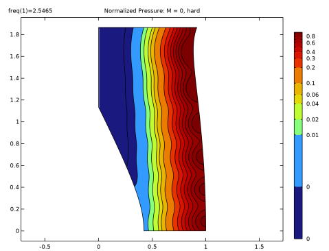
In the Settings window for 2D Plot Group, type Normalized Pressure: M = 0, hard in the Label text field.
|
|
3
|
Locate the Data section. From the Dataset list, choose Study 3 - Frequency Domain (M = 0, hard)/Solution 3 (sol3).
|
|
4
|
|
1
|
|
2
|
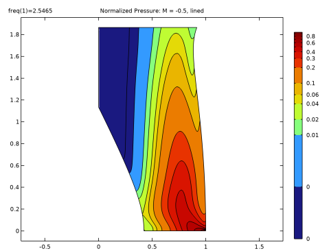
In the Settings window for 2D Plot Group, type Normalized Pressure: M = -0.5, lined in the Label text field.
|
|
3
|
Locate the Data section. From the Dataset list, choose Study 4 - Frequency Domain (M = -0.5, lined)/Solution 4 (sol4).
|
|
4
|
|
1
|
|
2
|
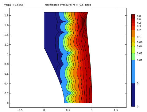
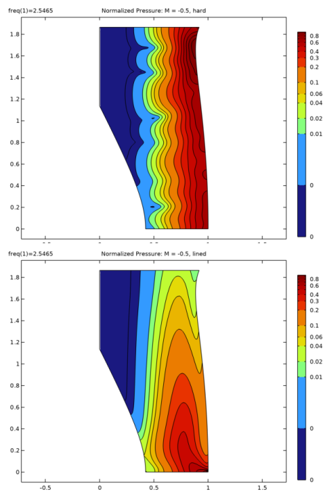
In the Settings window for 2D Plot Group, type Normalized Pressure: M = -0.5, hard in the Label text field.
|
|
3
|
Locate the Data section. From the Dataset list, choose Study 5 - Frequency Domain (M = -0.5, hard)/Solution 5 (sol5).
|
|
4
|
|
1
|
|
2
|
|
3
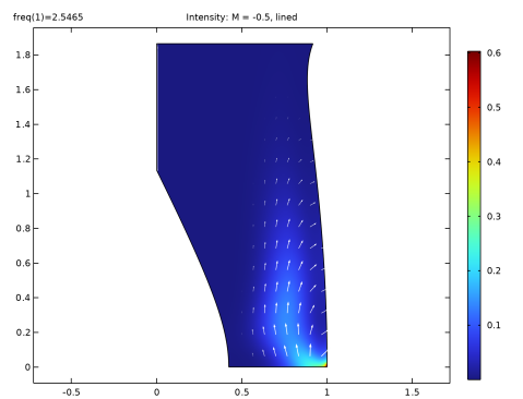
|
Click to expand the Selection section. Locate the Data section. From the Dataset list, choose Study 4 - Frequency Domain (M = -0.5, lined)/Solution 4 (sol4).
|
|
4
|
|
6
|
Select the Apply to dataset edges checkbox.
|
|
7
|
|
1
|
|
2
|
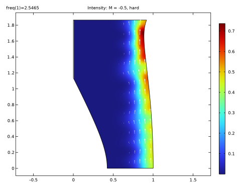
In the Settings window for Surface, click Replace Expression in the upper-right corner of the Expression section. From the menu, choose Component 1 (comp1) > Linearized Potential Flow, Frequency Domain > Intensity > lpff.I_mag - Intensity magnitude - kg/s³.
|
|
1
|
|
2
|
In the Settings window for Arrow Surface, click Replace Expression in the upper-right corner of the Expression section. From the menu, choose Component 1 (comp1) > Linearized Potential Flow, Frequency Domain > Intensity > lpff.Ir,lpff.Iz - Intensity.
|
|
3
|
|
4
|
|
5
|
|
6
|
|
1
|
|
2
|
|
3
|
Locate the Data section. From the Dataset list, choose Study 5 - Frequency Domain (M = -0.5, hard)/Solution 5 (sol5).
|
|
4
|
|
1
|
|
2
|
In the Settings window for Evaluation Group, type Evaluation Group: Attenuation in the Label text field.
|
|
3
|
|
1
|
|
2
|
|
3
|
|
4
|
Locate the Expressions section. In the table, enter the following settings:
|
|
1
|
In the Model Builder window, right-click Evaluation Group: Attenuation and choose Global Evaluation.
|
|
2
|
|
3
|
|
4
|
Locate the Expressions section. In the table, enter the following settings:
|
|
5
|