|
|
|
 ,
,

|
1
|
|
2
|
|
3
|
Click Add.
|
|
4
|
In the Select Physics tree, select Mathematics > PDE Interfaces > Lower Dimensions > Weak Form Boundary PDE (wb).
|
|
5
|
Click Add.
|
|
6
|
Click
|
|
7
|
|
8
|
Click
|
|
1
|
|
2
|
Browse to the model’s Application Libraries folder and double-click the file electric_motor_noise_pmsm_geom_sequence.mph.
|
|
3
|
|
4
|
|
5
|
|
6
|
|
1
|
|
2
|
|
3
|
Clear the Create pairs checkbox.
|
|
1
|
|
2
|
|
1
|
|
2
|
|
3
|
|
4
|
Browse to the model’s Application Libraries folder and double-click the file electric_motor_noise_pmsm_parameters.txt.
|
|
1
|
|
2
|
|
1
|
|
2
|
|
3
|
|
4
|
|
1
|
|
2
|
|
1
|
|
2
|
|
1
|
|
2
|
|
1
|
|
2
|
|
1
|
|
2
|
|
3
|
|
4
|
|
5
|
Click OK.
|
|
1
|
|
2
|
|
1
|
|
2
|
|
3
|
|
4
|
|
5
|
Click OK.
|
|
1
|
|
2
|
|
3
|
|
4
|
|
5
|
Click OK.
|
|
1
|
|
2
|
|
3
|
|
4
|
|
5
|
Click OK.
|
|
1
|
|
2
|
|
1
|
|
2
|
|
1
|
|
2
|
|
1
|
|
2
|
|
3
|
|
4
|
|
5
|
Click OK.
|
|
1
|
|
2
|
|
1
|
|
2
|
|
1
|
|
2
|
|
1
|
|
2
|
|
3
|
|
4
|
In the Add dialog, in the Selections to add list, choose Inner air gap, Outer air gap, and Exterior air.
|
|
5
|
Click OK.
|
|
1
|
|
2
|
|
3
|
|
4
|
|
5
|
Click OK.
|
|
6
|
|
7
|
|
8
|
|
9
|
Click OK.
|
|
1
|
|
2
|
|
3
|
|
4
|
|
5
|
|
1
|
|
2
|
|
3
|
|
4
|
|
5
|
Click OK.
|
|
1
|
|
2
|
|
3
|
|
4
|
|
5
|
Click OK.
|
|
1
|
|
2
|
|
3
|
|
4
|
|
5
|
In the Add dialog, in the Selections to add list, choose Adjacent to rotor forces and Adjacent to stator forces.
|
|
6
|
Click OK.
|
|
7
|
|
8
|
|
9
|
|
10
|
Click OK.
|
|
1
|
|
2
|
|
3
|
|
4
|
|
5
|
Click OK.
|
|
1
|
|
2
|
|
3
|
|
4
|
|
5
|
Click OK.
|
|
1
|
|
2
|
|
3
|
|
4
|
|
5
|
Click OK.
|
|
1
|
|
2
|
In the Settings window for Difference, type Adjacent to air gap in the stator in the Label text field.
|
|
3
|
|
4
|
|
5
|
|
6
|
Click OK.
|
|
7
|
|
8
|
|
9
|
|
10
|
Click OK.
|
|
1
|
In the Model Builder window, under Component 1 (comp1) right-click Definitions and choose Variables.
|
|
2
|
|
1
|
|
2
|
|
3
|
|
4
|
|
5
|
|
6
|
|
7
|
|
8
|
|
9
|
Select the Use NaN when mapping fails checkbox.
|
|
1
|
|
2
|
|
3
|
|
4
|
|
1
|
|
2
|
Go to the Add Material window.
|
|
3
|
|
4
|
Click the Add to Component button in the window toolbar.
|
|
1
|
|
2
|
|
1
|
Go to the Add Material window.
|
|
2
|
|
3
|
Click the Add to Component button in the window toolbar.
|
|
1
|
|
2
|
|
1
|
Go to the Add Material window.
|
|
2
|
In the tree, select AC/DC > Hard Magnetic Materials > Sintered NdFeB Grades (Chinese Standard) > N40 (Sintered NdFeB).
|
|
3
|
Click the Add to Component button in the window toolbar.
|
|
4
|
|
5
|
Click the Add to Component button in the window toolbar.
|
|
6
|
|
1
|
|
2
|
|
1
|
|
2
|
|
3
|
|
1
|
|
2
|
|
3
|
|
4
|
|
1
|
|
2
|
|
3
|
|
4
|
|
1
|
|
2
|
|
3
|
|
4
|
Locate the Coordinate System Selection section. From the Coordinate system list, choose Cylindrical System 3 (sys3).
|
|
5
|
Locate the Constitutive Relation B-H section. From the Magnetization model list, choose Remanent flux density.
|
|
6
|
|
1
|
|
2
|
|
3
|
|
4
|
|
1
|
|
2
|
|
3
|
|
4
|
|
5
|
|
6
|
Select the Coil group checkbox.
|
|
7
|
|
8
|
|
9
|
From the list, choose User defined.
|
|
10
|
|
11
|
|
1
|
|
1
|
|
2
|
|
3
|
|
4
|
|
1
|
|
2
|
|
3
|
Click
|
|
1
|
|
2
|
|
3
|
|
4
|
|
1
|
|
2
|
|
3
|
Click
|
|
1
|
|
2
|
|
3
|
Click
|
|
4
|
|
5
|
Click OK.
|
|
6
|
|
7
|
In the Show More Options dialog, in the tree, select the checkbox for the node Physics > Advanced Physics Options.
|
|
8
|
Click OK.
|
|
9
|
|
10
|
|
1
|
|
2
|
|
3
|
|
4
|
|
1
|
|
2
|
In the Settings window for Force Calculation, type Force Calculation Stator in the Label text field.
|
|
3
|
|
4
|
|
1
|
|
2
|
|
3
|
|
4
|
|
5
|
Click to expand the Dependent Variables section. In the Number of dependent variables text field, type 2.
|
|
6
|
In the Dependent variables (1) table, enter the following settings:
|
|
7
|
|
8
|
In the Dependent variable quantity table, enter the following settings:
|
|
9
|
Click
|
|
10
|
In the Source term quantity table, enter the following settings:
|
|
1
|
In the Model Builder window, under Component 1 (comp1) > Weak Form Boundary PDE (wb) click Initial Values 1.
|
|
2
|
|
3
|
In the Fx text field, type if(isnan(mf.nTx_stat),mf.nTx_rot*cos(rotation)+mf.nTy_rot*sin(rotation),mf.nTx_stat).
|
|
4
|
In the Fy text field, type if(isnan(mf.nTy_stat),-mf.nTx_rot*sin(rotation)+mf.nTy_rot*cos(rotation),mf.nTy_stat).
|
|
1
|
|
2
|
|
3
|
Click the Custom button.
|
|
4
|
|
5
|
|
6
|
|
7
|
|
1
|
|
2
|
|
3
|
|
4
|
|
5
|
|
6
|
Locate the Element Size Parameters section.
|
|
7
|
|
8
|
|
9
|
|
10
|
|
11
|
Click
|
|
1
|
|
2
|
|
3
|
Clear the Smooth transition to interior mesh checkbox.
|
|
1
|
|
2
|
|
3
|
|
4
|
|
5
|
Click
|
|
6
|
|
1
|
|
2
|
|
3
|
|
4
|
Locate the Physics and Variables Selection section. In the Solve for column of the table, under Component 1 (comp1), clear the checkbox for Weak Form Boundary PDE (wb).
|
|
5
|
Click to expand the Values of Dependent Variables section. Find the Initial values of variables solved for subsection. From the Settings list, choose User controlled.
|
|
6
|
|
7
|
|
8
|
Click to expand the Mesh Selection section. There is no need to use the mesh coming from the second component.
|
|
1
|
|
2
|
|
3
|
In the Solve for column of the table, under Component 1 (comp1), clear the checkbox for Weak Form Boundary PDE (wb).
|
|
4
|
Click to expand the Mesh Selection section. There is no need to use the mesh coming from the second component.
|
|
6
|
|
7
|
|
1
|
|
2
|
|
3
|
In the Model Builder window, expand the Study 1 - Electromagnetic Analysis > Solver Configurations > Solution 1 (sol1) > Time-Dependent Solver 1 node, then click Fully Coupled 1.
|
|
4
|
|
5
|
|
6
|
|
1
|
In the Model Builder window, expand the Results > Magnetic Flux Density (mf) node, then click Surface 1.
|
|
2
|
|
3
|
Select the Manual color range checkbox.
|
|
4
|
|
5
|
|
1
|
|
2
|
|
3
|
|
4
|
|
1
|
|
2
|
|
3
|
|
4
|
|
5
|
|
6
|
|
1
|
|
2
|
|
3
|
|
4
|
|
5
|
|
6
|
|
7
|
|
8
|
|
1
|
|
2
|
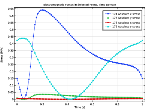
In the Settings window for 1D Plot Group, type Electromagnetic Forces in Selected Points, Time Domain in the Label text field.
|
|
3
|
Locate the Plot Settings section.
|
|
4
|
|
5
|
|
1
|
|
3
|
|
4
|
|
5
|
|
6
|
|
7
|
|
8
|
|
9
|
Click to expand the Coloring and Style section. Find the Line markers subsection. From the Marker list, choose Point.
|
|
10
|
|
1
|
|
2
|
|
3
|
|
4
|
|
1
|
|
2
|
|
3
|
Click
|
|
5
|
|
6
|
|
1
|
|
2
|
|
3
|
|
4
|
|
5
|
|
1
|
In the Model Builder window, right-click Electromagnetic Forces in Selected Points, Time Domain and choose Duplicate.
|
|
2
|
|
3
|
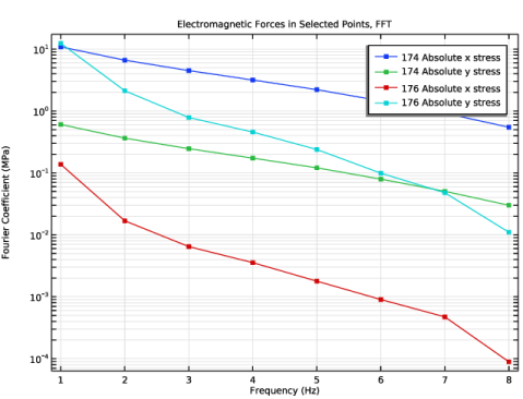
In the Settings window for 1D Plot Group, type Electromagnetic Forces in Selected Points, FFT in the Label text field.
|
|
4
|
Locate the Plot Settings section.
|
|
5
|
|
6
|
|
1
|
|
2
|
|
3
|
|
4
|
|
5
|
Select the Frequency range checkbox.
|
|
6
|
|
7
|
|
1
|
|
2
|
|
3
|
|
4
|
|
5
|
Select the Frequency range checkbox.
|
|
6
|
|
7
|
|
1
|
|
2
|
|
3
|
|
4
|
|
5
|
Select the Frequency range checkbox.
|
|
6
|
|
7
|
|
1
|
|
2
|
|
3
|
|
4
|
|
5
|
Select the Frequency range checkbox.
|
|
6
|
|
7
|
|
8
|
|
9
|
|
1
|
In the Model Builder window, right-click Electromagnetic Forces in Selected Points, FFT and choose Duplicate.
|
|
2
|
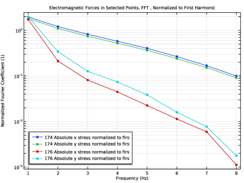
In the Settings window for 1D Plot Group, type Electromagnetic Forces in Selected Points, FFT , Normalized to First Harmonic in the Label text field.
|
|
3
|
Locate the Plot Settings section. In the y-axis label text field, type Normalized Fourier Coefficient (1).
|
|
4
|
|
1
|
In the Model Builder window, expand the Electromagnetic Forces in Selected Points, FFT , Normalized to First Harmonic node, then click Point Graph 1.
|
|
2
|
|
3
|
|
4
|
|
1
|
|
2
|
|
3
|
|
4
|
|
1
|
|
2
|
|
3
|
|
4
|
|
1
|
|
2
|
|
3
|
|
4
|
|
5
|
In the Electromagnetic Forces in Selected Points, FFT , Normalized to First Harmonic toolbar, click
|
|
1
|
|
2
|
Go to the Add Study window.
|
|
3
|
|
4
|
Click the Add Study button in the window toolbar.
|
|
5
|
|
1
|
|
2
|
|
3
|
|
4
|
|
5
|
|
6
|
|
7
|
Locate the Physics and Variables Selection section. In the Solve for column of the table, under Component 1 (comp1), clear the checkbox for Magnetic Fields (mf).
|
|
8
|
|
1
|
|
2
|
|
1
|
|
2
|
|
3
|
|
4
|
|
5
|
|
6
|
Select the Radius scale factor checkbox.
|
|
7
|
|
8
|
|
1
|
|
2
|
|
3
|
|
4
|
|
5
|
|
6
|
|
7
|
|
1
|
|
2
|
|
3
|
|
4
|
|
5
|
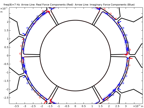
Select the Description checkbox. In the associated text field, type Imaginary Force Components (Blue).
|
|
6
|
|
7
|
|
8
|
|
1
|
In the Model Builder window, under Results, Ctrl-click to select Magnetic Flux Density (mf), Electromagnetic Forces in Selected Points, Time Domain, Electromagnetic Forces in Selected Points, FFT, Electromagnetic Forces in Selected Points, FFT , Normalized to First Harmonic, and Electromagnetic Forces, FFT.
|
|
2
|
Right-click and choose Group.
|
|
1
|
|
1
|
|
2
|
Go to the Add Physics window.
|
|
3
|
Find the Physics interfaces in study subsection. In the table, clear the Solve checkboxes for Study 1 - Electromagnetic Analysis and Study 2 - Electromagnetic Forces FFT.
|
|
4
|
In the tree, select Acoustics > Acoustic–Structure Interaction > Acoustic–Solid Interaction, Frequency Domain.
|
|
5
|
Click the Add to Component 2 button in the window toolbar.
|
|
6
|
|
1
|
In the Settings window for Pressure Acoustics, Frequency Domain, locate the Domain Selection section.
|
|
2
|
|
1
|
|
2
|
|
3
|
|
4
|
Locate the Exterior Field Calculation section. From the Condition in the z = z0 plane list, choose Symmetric/Infinite sound hard boundary.
|
|
5
|
|
1
|
|
2
|
|
3
|
|
1
|
|
2
|
|
3
|
|
1
|
|
2
|
|
3
|
|
4
|
|
5
|
|
6
|
|
7
|
|
1
|
|
2
|
|
3
|
|
4
|
|
1
|
|
2
|
|
3
|
|
1
|
|
2
|
|
3
|
|
4
|
|
5
|
Click
|
|
1
|
|
2
|
|
3
|
Click the Custom button.
|
|
4
|
Locate the Element Size Parameters section.
|
|
5
|
|
6
|
|
7
|
|
8
|
|
10
|
Click
|
|
1
|
|
3
|
|
4
|
Click to select the
|
|
6
|
Click
|
|
1
|
|
2
|
|
3
|
|
4
|
|
5
|
Click
|
|
1
|
|
2
|
|
3
|
|
4
|
|
5
|
Click
|
|
1
|
|
2
|
|
3
|
|
4
|
|
1
|
|
2
|
|
3
|
|
4
|
Click
|
|
1
|
|
2
|
|
3
|
|
5
|
|
1
|
|
2
|
|
3
|
|
4
|
|
5
|
Click
|
|
6
|
|
1
|
In the Model Builder window, under Component 2 (comp2) right-click Definitions and choose Variables.
|
|
2
|
|
1
|
|
2
|
|
3
|
|
4
|
|
5
|
|
6
|
Locate the Units section. In the table, enter the following settings:
|
|
7
|
|
8
|
Locate the Plot Parameters section. In the table, enter the following settings:
|
|
9
|
Click
|
|
1
|
|
2
|
|
3
|
|
4
|
|
5
|
|
6
|
Locate the Units section. In the table, enter the following settings:
|
|
7
|
|
8
|
Locate the Plot Parameters section. In the table, enter the following settings:
|
|
9
|
Click
|
|
1
|
|
2
|
|
3
|
|
4
|
|
1
|
|
2
|
Go to the Add Material window.
|
|
3
|
|
4
|
Click the Add to Component button in the window toolbar.
|
|
5
|
|
6
|
Click the Add to Component button in the window toolbar.
|
|
7
|
|
8
|
Click the Add to Component button in the window toolbar.
|
|
9
|
|
1
|
|
2
|
|
1
|
|
2
|
|
3
|
|
1
|
|
2
|
|
3
|
|
1
|
|
2
|
|
3
|
|
4
|
Locate the Material Contents section. In the table, enter the following settings:
|
|
1
|
|
2
|
Go to the Add Study window.
|
|
3
|
Find the Physics interfaces in study subsection. In the table, clear the Solve checkboxes for Magnetic Fields (mf) and Weak Form Boundary PDE (wb).
|
|
4
|
|
5
|
Click the Add Study button in the window toolbar.
|
|
6
|
|
1
|
|
2
|
In the Frequencies text field, type range(360[deg]/theta*rpm_idle*harm_exc,fdelta,min(fmax,rpm_max/rpm0*f0*harm_exc)) min(fmax,rpm_max/rpm0*f0*harm_exc).
|
|
3
|
Click to expand the Store in Output section. In the table, enter the following settings:
|
|
5
|
|
6
|
|
7
|
Click OK.
|
|
8
|
|
11
|
|
12
|
|
13
|
Click OK.
|
|
14
|
|
15
|
In the Settings window for Study, type Study 3 - Vibroacoustic Analysis - all Harmonics and Frequencies in the Label text field.
|
|
16
|
|
1
|
|
2
|
|
3
|
Click
|
|
1
|
|
2
|
|
3
|
In the Model Builder window, expand the Study 3 - Vibroacoustic Analysis - all Harmonics and Frequencies > Solver Configurations > Solution 4 (sol4) > Stationary Solver 1 node.
|
|
4
|
Right-click Study 3 - Vibroacoustic Analysis - all Harmonics and Frequencies > Solver Configurations > Solution 4 (sol4) > Stationary Solver 1 and choose Segregated.
|
|
5
|
|
6
|
|
7
|
In the Model Builder window, expand the Study 3 - Vibroacoustic Analysis - all Harmonics and Frequencies > Solver Configurations > Solution 4 (sol4) > Stationary Solver 1 > Segregated 1 node, then click Segregated Step.
|
|
8
|
|
9
|
|
10
|
|
11
|
In the Model Builder window, under Study 3 - Vibroacoustic Analysis - all Harmonics and Frequencies > Solver Configurations > Solution 4 (sol4) > Stationary Solver 1 right-click Segregated 1 and choose Segregated Step.
|
|
12
|
|
13
|
|
14
|
|
15
|
Click OK.
|
|
16
|
In the Model Builder window, under Study 3 - Vibroacoustic Analysis - all Harmonics and Frequencies > Solver Configurations > Solution 4 (sol4) > Stationary Solver 1 click Suggested Direct Solver (asb1).
|
|
17
|
|
18
|
|
19
|
In the Model Builder window, click Study 3 - Vibroacoustic Analysis - all Harmonics and Frequencies.
|
|
20
|
|
21
|
Clear the Generate convergence plots checkbox.
|
|
22
|
|
1
|
In the Model Builder window, under Results > Datasets, Ctrl-click to select Study 3 - Vibroacoustic Analysis - all Harmonics and Frequencies/Solution 4 (4) (sol4), Study 3 - Vibroacoustic Analysis - all Harmonics and Frequencies/Solution 4 (5) (sol4), and Study 3 - Vibroacoustic Analysis - all Harmonics and Frequencies/Parametric Solutions 1 (6) (sol5).
|
|
2
|
Right-click and choose Delete.
|
|
1
|
|
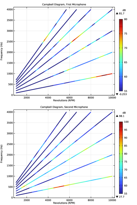
2
|
In the Settings window for 1D Plot Group, type Campbell Diagram, First Microphone in the Label text field.
|
|
3
|
Locate the Data section. From the Dataset list, choose Study 3 - Vibroacoustic Analysis - all Harmonics and Frequencies/Parametric Solutions 1 (sol5).
|
|
4
|
|
1
|
|
2
|
|
4
|
|
5
|
|
6
|
|
7
|
|
8
|
|
1
|
|
2
|
|
3
|
|
4
|
|
5
|
|
6
|
|
7
|
|
8
|
|
1
|
|
2
|
|
3
|
Select the Show maximum and minimum values checkbox.
|
|
4
|
Select the Show units checkbox.
|
|
5
|
|
1
|
|
2
|
|
3
|
In the Settings window for 1D Plot Group, type Campbell Diagram, Second Microphone in the Label text field.
|
|
1
|
In the Model Builder window, expand the Results > Campbell Diagram, Second Microphone > Global 1 node, then click Color Expression 1.
|
|
2
|
|
3
|
|
4
|
|
5
|
|
1
|
|
2
|
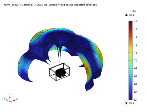
In the Settings window for 3D Plot Group, type Exterior-Field Sound Pressure Level (acpr) in the Label text field.
|
|
3
|
|
4
|
|
5
|
|
6
|
Select the Show units checkbox.
|
|
1
|
In the Exterior-Field Sound Pressure Level (acpr) toolbar, click
|
|
2
|
|
3
|
|
4
|
Select the Description checkbox. In the associated text field, type Exterior-field sound pressure level.
|
|
5
|
Clear the Use as color expression checkbox.
|
|
6
|
|
7
|
|
8
|
|
9
|
Locate the Evaluation section. Find the Angles subsection. In the Number of elevation angles text field, type 160.
|
|
10
|
|
11
|
|
12
|
|
13
|
|
14
|
|
15
|
|
16
|
|
17
|
|
18
|
|
1
|
|
2
|
|
3
|
Select the Plot dataset edges checkbox.
|
|
4
|
|
5
|
|
1
|
In the Model Builder window, under Results, Ctrl-click to select Campbell Diagram, First Microphone, Campbell Diagram, Second Microphone, and Exterior-Field Sound Pressure Level (acpr).
|
|
2
|
Right-click and choose Group.
|
|
1
|
|
2
|
In the Settings window for Evaluation Group, type Pressure - Revolutions - 1st Harmonic in the Label text field.
|
|
3
|
Locate the Data section. From the Dataset list, choose Study 3 - Vibroacoustic Analysis - all Harmonics and Frequencies/Parametric Solutions 1 (sol5).
|
|
4
|
|
5
|
|
6
|
|
1
|
|
2
|
|
4
|
|
1
|
In the Model Builder window, right-click Pressure - Revolutions - 1st Harmonic and choose Duplicate.
|
|
2
|
In the Settings window for Evaluation Group, type Pressure - Revolutions - 2nd Harmonic in the Label text field.
|
|
3
|
|
4
|
|
1
|
|
2
|
In the Settings window for Evaluation Group, type Pressure - Revolutions - 3rd Harmonic in the Label text field.
|
|
3
|
|
4
|
|
1
|
|
2
|
In the Settings window for Evaluation Group, type Pressure - Revolutions - 4th Harmonic in the Label text field.
|
|
3
|
|
4
|
|
1
|
|
2
|
In the Settings window for Evaluation Group, type Pressure - Revolutions - 5th Harmonic in the Label text field.
|
|
3
|
|
4
|
|
1
|
|
2
|
In the Settings window for Evaluation Group, type Pressure - Revolutions - 6th Harmonic in the Label text field.
|
|
3
|
|
4
|
|
1
|
|
2
|
In the Settings window for Evaluation Group, type Pressure - Revolutions - 7th Harmonic in the Label text field.
|
|
3
|
|
4
|
|
1
|
In the Model Builder window, under Results, Ctrl-click to select Pressure - Revolutions - 1st Harmonic, Pressure - Revolutions - 2nd Harmonic, Pressure - Revolutions - 3rd Harmonic, Pressure - Revolutions - 4th Harmonic, Pressure - Revolutions - 5th Harmonic, Pressure - Revolutions - 6th Harmonic, and Pressure - Revolutions - 7th Harmonic.
|
|
2
|
Right-click and choose Group.
|
|
1
|
|
2
|
|
3
|
|
4
|
Locate the Data Column Settings section. In the table, enter the following settings:
|
|
6
|
|
8
|
|
9
|
|
11
|
|
12
|
|
14
|
|
15
|
|
17
|
|
18
|
|
19
|
Locate the Interpolation and Extrapolation section. From the Interpolation list, choose Piecewise cubic.
|
|
20
|
|
21
|
Click
|
|
1
|
|
2
|
|
3
|
|
4
|
Locate the Data Column Settings section. In the table, click to select the cell at row number 2 and column number 1.
|
|
5
|
|
7
|
|
9
|
|
11
|
|
12
|
Click
|
|
1
|
|
2
|
|
3
|
|
4
|
Locate the Data Column Settings section. In the table, click to select the cell at row number 2 and column number 1.
|
|
5
|
|
7
|
|
9
|
|
11
|
|
12
|
Click
|
|
1
|
|
2
|
|
3
|
|
4
|
Locate the Data Column Settings section. In the table, click to select the cell at row number 2 and column number 1.
|
|
5
|
|
7
|
|
9
|
|
11
|
|
12
|
Click
|
|
1
|
|
2
|
|
3
|
|
4
|
Locate the Data Column Settings section. In the table, click to select the cell at row number 2 and column number 1.
|
|
5
|
|
7
|
|
9
|
|
11
|
|
12
|
Click
|
|
1
|
|
2
|
|
3
|
|
4
|
Locate the Data Column Settings section. In the table, click to select the cell at row number 2 and column number 1.
|
|
5
|
|
7
|
|
9
|
|
11
|
|
12
|
Click
|
|
1
|
|
2
|
|
3
|
|
4
|
Locate the Data Column Settings section. In the table, click to select the cell at row number 2 and column number 1.
|
|
5
|
|
7
|
|
9
|
|
11
|
|
12
|
Click
|
|
1
|
In the Model Builder window, under Component 2 (comp2) > Definitions, Ctrl-click to select Interpolation 1 (real1_l, imag1_l, ...), Interpolation 2 (real2_l, imag2_l, ...), Interpolation 3 (real3_l, imag3_l, ...), Interpolation 4 (real4_l, imag4_l, ...), Interpolation 5 (real5_l, imag5_l, ...), Interpolation 6 (real6_l, imag6_l, ...), and Interpolation 7 (real7_l, imag7_l, ...).
|
|
2
|
Right-click and choose Group.
|
|
1
|
|
2
|
Go to the Add Study window.
|
|
3
|
Find the Physics interfaces in study subsection. In the table, clear the Solve checkboxes for Magnetic Fields (mf) and Weak Form Boundary PDE (wb).
|
|
4
|
|
5
|
Click the Add Study button in the window toolbar.
|
|
6
|
|
1
|
|
2
|
|
3
|
|
4
|
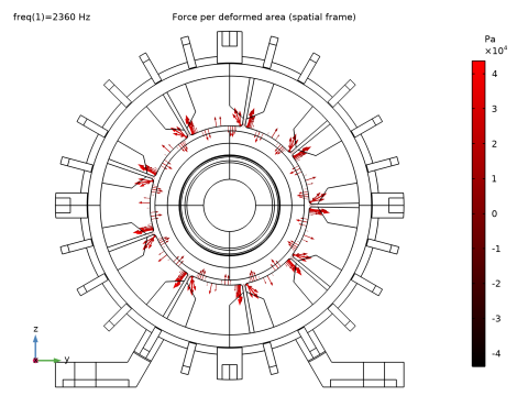
In the Settings window for Study, type Study 4 - Vibroacoustic Analysis - 3rd Harmonic 2360 Hz in the Label text field.
|
|
5
|
|
6
|
Clear the Generate convergence plots checkbox.
|
|
1
|
|
2
|
|
3
|
In the Model Builder window, expand the Study 4 - Vibroacoustic Analysis - 3rd Harmonic 2360 Hz > Solver Configurations > Solution 13 (sol13) > Stationary Solver 1 node.
|
|
4
|
Right-click Study 4 - Vibroacoustic Analysis - 3rd Harmonic 2360 Hz > Solver Configurations > Solution 13 (sol13) > Stationary Solver 1 and choose Segregated.
|
|
5
|
|
6
|
|
7
|
In the Model Builder window, expand the Study 4 - Vibroacoustic Analysis - 3rd Harmonic 2360 Hz > Solver Configurations > Solution 13 (sol13) > Stationary Solver 1 > Segregated 1 node, then click Segregated Step.
|
|
8
|
|
9
|
|
10
|
|
11
|
In the Model Builder window, under Study 4 - Vibroacoustic Analysis - 3rd Harmonic 2360 Hz > Solver Configurations > Solution 13 (sol13) > Stationary Solver 1 right-click Segregated 1 and choose Segregated Step.
|
|
12
|
|
13
|
|
14
|
|
15
|
Click OK.
|
|
16
|
|
1
|
|
2
|
|
3
|
From the Dataset list, choose Study 4 - Vibroacoustic Analysis - 3rd Harmonic 2360 Hz/Solution 13 (sol13).
|
|
4
|
|
5
|
|
6
|
|
1
|
|
2
|
|
3
|
|
4
|
|
5
|
Locate the Plot Settings section.
|
|
6
|
|
1
|
|
2
|
|
3
|
Locate the y-Axis Data section.
|
|
4
|
|
5
|
In the Expression text field, type real((real1_l(rev_ramp(tt))+i*imag1_l(rev_ramp(tt)))*exp(i*(rev_ramp(tt))*f0/rpm0*1*pi*tt)+(real2_l(rev_ramp(tt))+i*imag2_l(rev_ramp(tt)))*exp(i*(rev_ramp(tt))*f0/rpm0*2*pi*tt)+(real3_l(rev_ramp(tt))+i*imag3_l(rev_ramp(tt)))*exp(i*(rev_ramp(tt))*f0/rpm0*3*pi*tt)+(real4_l(rev_ramp(tt))+i*imag4_l(rev_ramp(tt)))*exp(i*(rev_ramp(tt))*f0/rpm0*4*pi*tt)+(real5_l(rev_ramp(tt))+i*imag5_l(rev_ramp(tt)))*exp(i*(rev_ramp(tt))*f0/rpm0*5*pi*tt)+(real6_l(rev_ramp(tt))+i*imag6_l(rev_ramp(tt)))*exp(i*(rev_ramp(tt))*f0/rpm0*6*pi*tt)+(real7_l(rev_ramp(tt))+i*imag7_l(rev_ramp(tt)))*exp(i*(rev_ramp(tt))*f0/rpm0*7*pi*tt)).
|
|
6
|
|
7
|
|
8
|
|
9
|
|
10
|
|
11
|
Select the Label checkbox.
|
|
12
|
|
1
|
|
2
|
|
3
|
|
4
|
In the Expression text field, type real((real1_r(rev_ramp(tt))+i*imag1_r(rev_ramp(tt)))*exp(i*(rev_ramp(tt))*f0/rpm0*1*pi*tt)+(real2_r(rev_ramp(tt))+i*imag2_r(rev_ramp(tt)))*exp(i*(rev_ramp(tt))*f0/rpm0*2*pi*tt)+(real3_r(rev_ramp(tt))+i*imag3_r(rev_ramp(tt)))*exp(i*(rev_ramp(tt))*f0/rpm0*3*pi*tt)+(real4_r(rev_ramp(tt))+i*imag4_r(rev_ramp(tt)))*exp(i*(rev_ramp(tt))*f0/rpm0*4*pi*tt)+(real5_r(rev_ramp(tt))+i*imag5_r(rev_ramp(tt)))*exp(i*(rev_ramp(tt))*f0/rpm0*5*pi*tt)+(real6_r(rev_ramp(tt))+i*imag6_r(rev_ramp(tt)))*exp(i*(rev_ramp(tt))*f0/rpm0*6*pi*tt)+(real7_r(rev_ramp(tt))+i*imag7_r(rev_ramp(tt)))*exp(i*(rev_ramp(tt))*f0/rpm0*7*pi*tt)).
|
|
5
|
|
6
|
|
1
|
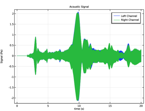
In the Model Builder window, under Results > Vibroacoustic Results - all Harmonics and Frequencies > Acoustic Signal right-click Left Channel and choose Add Plot Data to Export.
|
|
2
|
|
3
|
|
4
|
|
5
|
Click Export to produce a WAV-file with the acoustic signal at the left channel.
|
|
1
|
In the Model Builder window, under Results > Vibroacoustic Results - all Harmonics and Frequencies > Acoustic Signal right-click Right Channel and choose Add Plot Data to Export.
|
|
2
|
|
3
|
|
4
|
|
5
|
Click Export to produce a WAV-file with the acoustic signal at the right channel.
|
|
1
|
|
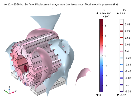
2
|
In the Settings window for 3D Plot Group, type Displacement and Acoustic Pressure in the Label text field.
|
|
3
|
Locate the Data section. From the Dataset list, choose Study 4 - Vibroacoustic Analysis - 3rd Harmonic 2360 Hz/Solution 13 (sol13).
|
|
4
|
|
5
|
|
6
|
Select the Show units checkbox.
|
|
1
|
|
2
|
|
3
|
|
1
|
|
2
|
|
3
|
|
4
|
|
1
|
|
2
|
|
3
|
|
4
|
|
5
|
|
6
|
|
1
|
|
2
|
|
3
|
Clear the Color checkbox.
|
|
4
|
Clear the Color and data range checkbox.
|
|
5
|
|
1
|
|
2
|
|
3
|
|
1
|
|
1
|
|
1
|
|
2
|
|
3
|
Locate the Data section. From the Dataset list, choose Study 4 - Vibroacoustic Analysis - 3rd Harmonic 2360 Hz/Solution 13 (sol13).
|
|
4
|
|
5
|
|
6
|
|
7
|
|
8
|
|
1
|
|
2
|
|
3
|
|
4
|
|
5
|
|
6
|
|
1
|
|
2
|
|
3
|
|
4
|
|
5
|
|
6
|
|
7
|
|
8
|
Clear the Color checkbox.
|
|
9
|
Clear the Color and data range checkbox.
|
|
1
|
In the Model Builder window, expand the Results > Vibroacoustic Results - all Harmonics and Frequencies > Exterior-Field Sound Pressure Level (acpr) node.
|
|
2
|
|
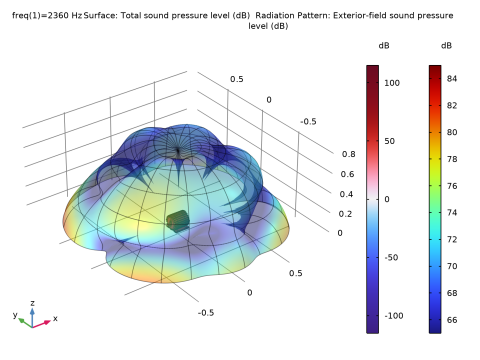
1
|
In the Model Builder window, right-click SPL and Radiation Pattern and choose Paste Radiation Pattern.
|
|
2
|
|
3
|
|
4
|
|
1
|
|
2
|
|
1
|
|
2
|
|
3
|
Locate the Data section. From the Dataset list, choose Study 4 - Vibroacoustic Analysis - 3rd Harmonic 2360 Hz/Solution 13 (sol13).
|
|
4
|
|
5
|
|
6
|
Select the Apply to dataset edges checkbox.
|
|
7
|
|
1
|
|
2
|
|
3
|
|
4
|
|
5
|
|
6
|
|
1
|
|
2
|
|
3
|
|
4
|
|
5
|
|
6
|
|
7
|
|
1
|
In the Model Builder window, under Results, Ctrl-click to select Displacement and Acoustic Pressure, SPL and Radiation Pattern, and Boundary Loads.
|
|
2
|
Right-click and choose Group.
|
|
1
|
|
2
|
Click
|
|
1
|
|
2
|
|
3
|
Click
|
|
4
|
Browse to the model’s Application Libraries folder and double-click the file electric_motor_noise_pmsm_geom_sequence_parameters.txt.
|
|
1
|
|
2
|
|
3
|
|
4
|
Click
|
|
5
|
Browse to the model’s Application Libraries folder and double-click the file electric_motor_noise_pmsm_geom_sequence.mphbin.
|
|
6
|
Click
|
|
7
|
|
1
|
|
2
|
|
3
|
|
4
|
|
5
|
|
6
|
On the object imp1, select Point 372 only.
|
|
1
|
|
2
|
|
3
|
|
4
|
Click to expand the Layers section. In the table, enter the following settings:
|
|
5
|
Click
|
|
1
|
|
2
|
|
4
|
Click
|
|
1
|
|
2
|
|
4
|
Click
|
|
1
|
|
2
|
|
3
|
|
1
|
|
2
|
On the object c1, select Boundaries 1–12 only.
|
|
3
|
On the object uni1, select Boundaries 1, 4, 5, and 12–14 only.
|
|
4
|
|
1
|
|
2
|
Select the object del1(2) only.
|
|
3
|
|
4
|
|
5
|
Click
|
|
1
|
|
2
|
Click in the Graphics window and then press Ctrl+A to select all objects.
|
|
3
|
|
1
|
|
2
|
On the object uni2, select Boundaries 75, 76, 83, 84, 91, 92, 99–102, 113, 114, 121–124, 127, 128, 135, and 136 only.
|
|
3
|
|
1
|
|
2
|
|
3
|
|
4
|
On the object del2, select Domain 21 only.
|
|
5
|
Click
|
|
1
|
|
2
|
On the object del3, select Points 22–25, 38–41, 54, 55, 58, 59, 70–73, 81, and 82 only.
|
|
3
|
|
4
|
|
5
|
Click
|
|
1
|
In the Model Builder window, under Component 1 (comp1) > Geometry 1 right-click Work Plane 1 (wp1) and choose Extrude.
|
|
2
|
|
3
|
|
4
|
On the object imp1, select Point 490 only.
|
|
5
|
Click
|
|
1
|
|
2
|
Click in the Graphics window and then press Ctrl+A to select both objects.
|
|
3
|
|
1
|
|
2
|
|
3
|
|
4
|
|
5
|
|
6
|
On the object uni1, select Point 422 only.
|
|
1
|
|
2
|
|
3
|
|
4
|
Locate the Layers section. In the table, enter the following settings:
|
|
5
|
Click
|
|
1
|
|
2
|
|
3
|
|
4
|
|
5
|
|
6
|
|
7
|
|
8
|
|
9
|
Click
|
|
1
|
|
2
|
Select the object ls1 only.
|
|
3
|
|
4
|
In the Angle text field, type range(360/(n_poles),360/(n_poles),360) range(360/(n_poles)+angle_magnet,360/(n_poles),360+angle_magnet).
|
|
5
|
Click
|
|
1
|
|
2
|
Select the object c1 only.
|
|
3
|
|
4
|
|
1
|
|
2
|
On the object uni1, select Boundaries 1, 2, 5, 10–15, 18, 23, 24, 27, 28, 35, 36, 57, 58, 63, and 64 only.
|
|
3
|
|
1
|
|
2
|
On the object del1, select Points 2, 3, 7–10, 29–32, 36, and 37 only.
|
|
3
|
|
4
|
|
5
|
Click
|
|
1
|
In the Model Builder window, under Component 1 (comp1) > Geometry 1 right-click Work Plane 2 (wp2) and choose Extrude.
|
|
2
|
|
3
|
|
4
|
On the object uni1, select Point 656 only.
|
|
5
|
Click
|
|
1
|
|
2
|
|
3
|
|
4
|
Click
|
|
1
|
|
2
|
|
3
|
|
4
|
|
1
|
|
2
|
|
3
|
On the object fin, select Domains 13, 24, and 49 only.
|
|
1
|
|
2
|
|
3
|
On the object fin, select Domains 25, 26, and 28–43 only.
|
|
1
|
|
2
|
|
3
|
On the object fin, select Domains 14–17, 19–22, 45–47, and 50–52 only.
|
|
1
|
|
2
|
|
3
|
|
4
|
|
5
|
Click OK.
|
|
1
|
|
2
|
|
3
|
On the object fin, select Domains 18, 23–44, 48, and 59–67 only.
|
|
1
|
|
2
|
|
3
|
On the object fin, select Domains 1–8, 10–12, and 53–58 only.
|
|
1
|
|
2
|
|
3
|
|
4
|
|
5
|
Click OK.
|
|
1
|
|
2
|
|
3
|
|
4
|
On the object fin, select Boundaries 335, 336, 338, 339, 347, 349, 352, 355, 359, 360, 366, 367, 371, 372, 374, 375, 377, 378, 380–385, 389–394, 396, 398, 401, 402, 404, 407, 413–422, 425–428, 438–441, 444, 446–448, 450, 451, 456, 457, 460–463, 466, 469–477, 486–495, 497, 498, 500, 501, 506, 509, 514–517, 520, 521, 523, 524, 526, 529, 532–537, and 553–556 only.
|
|
1
|
|
2
|
In the Settings window for Explicit Selection, type Exterior Field Calculation in the Label text field.
|
|
3
|
|
4
|
On the object fin, select Boundaries 31, 32, 36, 39, and 924 only.
|
|
1
|
|
2
|
|
3
|
|
4
|
On the object fin, select Boundaries 213, 214, 217, 247, 249, 257, 291, 292, 294–297, 299, 300, 581, 582, 597, 690, 692, 719, 725, 726, 728–731, 733, and 734 only.
|
|
1
|
|
2
|
|
3
|
|
4
|
On the object fin, select Boundaries 301, 306, 317, 331, 334, 337, 351, 354, 376, 379, 403, 406, 431, 437, 445, 464, 467, 496, 499, 505, 508, 525, 528, 538, 949, 952, 957, 966, 969, 976, 993, and 996 only.
|
|
1
|
|
2
|
|
3
|
On the object fin, select Domains 13, 21–26, 28–44, 49, and 60–67 only.
|
|
1
|
|
2
|
|
3
|
|
4
|
|
5
|
Click OK.
|