PDF

Eigenmodes in a Muffler with Elastic Walls
Introduction
This model is an extension of the model Eigenmodes in a Muffler. The latter studies the propagation of acoustic waves through the cross section of the Absorptive Muffler chamber, provided that the muffler walls were sound hard. Here the muffler walls are considered to be made of a linear elastic material to account for their influence on the modes propagating through the cross section of the chamber. This is done using the Acoustic–Solid Interaction, Frequency Domain multiphysics interface. The Mode following functionality is used to compute the dispersion diagram for the two configurations.
Model Definition
The muffler chamber has the same shape and dimensions as in example (Eigenmodes in a Muffler). The only difference is that an elastic wall of the thickness W surrounds the inner (acoustic) domain as shown in Figure 1.
Figure 1: Geometry of model: the chamber of the same cross section as in Eigenmodes in a Muffler with the elastic wall to the thickness W.
The chamber is filled with air and the elastic wall is made of steel. Assuming the time-harmonic process with the angular frequency ω = 2π·f, the Mode Analysis study solves the equations for the out-of-plane wave number κz as the function of given parameter f. The cutoff frequency for the j-th mode is then calculated as
(1)
Results and Discussion
The results of the simulations show that the presence of a thin elastic wall significantly affects the number of modes propagating through the cross section of the chamber. It becomes greater than that for the chamber with the sound hard wall boundary studied in the model Eigenmodes in a Muffler. For example, the first propagating mode with the wave number lower than that of the plane wave mode has its cutoff frequency around 218 Hz. The former mode is shown in Figure 2; the latter, in Figure 3. Both figures shows the acoustic pressure in the chamber and the deformation of the muffler wall.
Figure 2: The plane wave propagating through the cross section of the chamber.
Figure 3: The first propagating mode different from the plane wave.
The model Eigenmodes in a Muffler gives the first least nonzero cutoff frequency equal to 635 Hz. A good understanding of the difference between these two cases is provided by the dispersion diagrams shown in Figure 4. The top figure shows the diagram for the system with elastic walls while the bottom figure is the case for the hard wall configuration.
Another feature that distinguishes the chamber with the wall is that there can be modes having the wave number greater than that for the plane-wave mode, which is due to acoustics-structure interaction. In Figure 5 at a frequency of 400 Hz the pure acoustic plane wave-number is 7.33 1/m (the actual plane wave mode is at 7.27 1/m). While the wave number selected has a value of 7.87 1/m. This corresponds to the point above the red dotted line at 400 Hz in Figure 4. This means that their cutoff frequencies fj calculated from Equation 1 become pure imaginary. Such modes do not exist in the model Eigenmodes in a Muffler.
.
Figure 4: Dispersion diagram for the elastic wall case (top) and the hard wall case (bottom).
Figure 5: A propagating mode with the wave number greater that of the plane wave.
Notes About the COMSOL Implementation
In this model Mode following is used when computing the dispersion diagram. It will ensure that a diagram can be plotted and modes are sorted and located in the same position in the list if Out-of-plane wave number when varying the outer parameter for the frequency f0.
Note that when plotting and referring to a dataset generated with the study that uses mode following, entries of the type Nan+inf*i can exist. These are “empty” solutions or placeholders that are filled as the frequency parameter increases and new modes appear.
Filtering is also used in this model for two cases:
Removing evanescent (non-propagating) modes using the logic expression: abs(imag(comp1.acpr.kz))/abs(comp1.acpr.kz) < 1e-3
This removes modes that have imaginary parts that is larger than a factor 1000 of the absolute value of the wave number.
Application Library path: Acoustics_Module/Automotive/eigenmodes_in_muffler_elastic
Modeling Instructions
From the File menu, choose New.
New
In the New window, click  Model Wizard.
Model Wizard
1
In the Model Wizard window, click  2D.
2
In the Select Physics tree, select Acoustics > Acoustic–Structure Interaction > Acoustic–Solid Interaction, Frequency Domain.
3
Click Add.
4
Click  Study.
5
In the Select Study tree, select Preset Studies for Selected Physics Interfaces > Mode Analysis.
6
Global Definitions
Parameters 1
1
In the Model Builder window, under Global Definitions click Parameters 1.
2
In the Settings window for Parameters, locate the Parameters section.
3
The parameter k0 stands for the wave number of the plane wave generated at the cutoff frequency f0: k0 = 2π/λ0 = 2πf0/c0.
Geometry 1
1
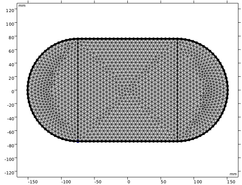
In the Model Builder window, expand the Component 1 (comp1) > Geometry 1 node, then click Geometry 1.
2
In the Settings window for Geometry, locate the Units section.
3
From the Length unit list, choose mm.
Rectangle 1 (r1)
1
In the Geometry toolbar, click  Rectangle.
2
In the Settings window for Rectangle, locate the Size and Shape section.
3
In the Width text field, type 150.
4
In the Height text field, type 150 + 2*W.
5
Locate the Position section. In the x text field, type -75.
6
In the y text field, type -75 - W.
7
Click to expand the Layers section. In the table, enter the following settings:
8
Select the Layers on top checkbox.
9
Click  Build Selected.
Circle 1 (c1)
1
In the Geometry toolbar, click  Circle.
2
In the Settings window for Circle, locate the Size and Shape section.
3
In the Radius text field, type 75 + W.
4
In the Sector angle text field, type 180.
5
Locate the Position section. In the x text field, type -75.
6
Locate the Rotation Angle section. In the Rotation text field, type 90.
7
Click to expand the Layers section. In the table, enter the following settings:
8
Click  Build Selected.
Circle 2 (c2)
1
In the Geometry toolbar, click  Circle.
2
In the Settings window for Circle, locate the Size and Shape section.
3
In the Radius text field, type 75 + W.
4
In the Sector angle text field, type 180.
5
Locate the Position section. In the x text field, type 75.
6
Locate the Rotation Angle section. In the Rotation text field, type -90.
7
Locate the Layers section. In the table, enter the following settings:
8
Click  Build Selected.
9
In the Geometry toolbar, click  Build All.
10
Click the  Zoom Extents button in the Graphics toolbar.
The geometry should look like the one in Figure 1.
Add Material
1
In the Materials toolbar, click  Add Material to open the Add Material window.
2
Go to the Add Material window.
3
In the tree, select Built-in > Air.
4
Click the Add to Component button in the window toolbar.
5
In the tree, select Built-in > Steel AISI 4340.
6
Click the Add to Component button in the window toolbar.
7
In the Materials toolbar, click  Add Material to close the Add Material window.
Materials
Steel AISI 4340 (mat2)
Select Domains 1–3, 6, 7, and 9 only.
Pressure Acoustics, Frequency Domain (acpr)
1
In the Model Builder window, under Component 1 (comp1) click Pressure Acoustics, Frequency Domain (acpr).
2
In the Settings window for Pressure Acoustics, Frequency Domain, locate the Domain Selection section.
3
From the Selection list, choose Manual.
4
Solid Mechanics (solid)
1
In the Model Builder window, under Component 1 (comp1) click Solid Mechanics (solid).
2
In the Settings window for Solid Mechanics, locate the Domain Selection section.
3
From the Selection list, choose Manual.
4
Enable the Out-of-plane mode extension (time-harmonic) to perform the Mode Analysis for elastic waves in the muffler wall domain.
5
Locate the 2D Approximation section. Select the Out-of-plane mode extension (time-harmonic) checkbox.
Mesh 1
In this model, the mesh is set up manually. Proceed by directly adding the desired mesh component.
Free Triangular 1
1
In the Mesh toolbar, click  Free Triangular.
2
In the Settings window for Free Triangular, locate the Domain Selection section.
3
From the Geometric entity level list, choose Domain.
4
Size 1
1
Right-click Free Triangular 1 and choose Size.
2
In the Settings window for Size, locate the Element Size section.
3
From the Predefined list, choose Extra fine.
Create a Mapped mesh for the muffler wall domain and choose the Distribution depth of 3 elements.
Mapped 1
1
In the Mesh toolbar, click  Mapped.
Use the Zoom Box functionality to investigate the boundary layer mesh.
Distribution 1
1
Right-click Mapped 1 and choose Distribution.
2
3
In the Settings window for Distribution, locate the Distribution section.
4
In the Number of elements text field, type 3.
5
Click  Build All.
Study 1
Step 1: Mode Analysis
1
In the Model Builder window, under Study 1 click Step 1: Mode Analysis.
2
In the Settings window for Mode Analysis, locate the Study Settings section.
3
In the Mode analysis frequency text field, type f0.
Set the solver to search for the first 6 propagating modes with the wave numbers lower that k0.
4
Select the Desired number of modes checkbox.
Search for the modes below the plane wave mode.
5
Select the Search for modes around shift checkbox. In the associated text field, type 1.1*k0.
6
From the Search method around shift list, choose Smaller real part.
7
In the Study toolbar, click  Compute.
Results
Acoustic Pressure (acpr)
Now, select the out-of-plane wave number with a value close to 5.18. This is the first nonplane mode.
1
In the Settings window for 2D Plot Group, locate the Data section.
2
From the Out-of-plane wave number (rad/m) list, choose 5.1756.
Surface 2
1
In the Model Builder window, right-click Acoustic Pressure (acpr) and choose Surface.
2
In the Settings window for Surface, locate the Expression section.
3
In the Expression text field, type solid.disp.
4
Locate the Coloring and Style section. From the Color table list, choose AuroraBorealis.
5
From the Scale list, choose Linear.
Deformation 1
1
Right-click Surface 2 and choose Deformation.
The results should look like the one depicted in Figure 3.
Dispersion Relation Calculation
The next steps are optional and are added to show you how to get the dispersion relation curves that relate the frequency and the wave number. The Mode following option is used for this analysis, it is found in the Filtering and Sorting section of the study step. The dispersion relations for the chamber with elastic and hard walls are calculated and compared below.
Add Study
1
In the Home toolbar, click  Add Study to open the Add Study window.
2
Go to the Add Study window.
3
Find the Studies subsection. In the Select Study tree, select Preset Studies for Selected Physics Interfaces > Mode Analysis.
4
Click the Add Study button in the window toolbar.
5
In the Home toolbar, click  Add Study to close the Add Study window.
Study 2
Step 1: Mode Analysis
1
In the Settings window for Mode Analysis, locate the Study Settings section.
2
In the Mode analysis frequency text field, type f0.
3
Select the Desired number of modes checkbox.
4
Select the Search for modes around shift checkbox.
5
In the Desired number of modes text field, type 12.
6
In the Search for modes around shift text field, type 1.2*k0.
Search, starting a bit higher than the plane wave mode and look for 12 modes.
7
From the Search method around shift list, choose Smaller real part.
8
Click to expand the Filtering and Sorting section. Find the Filtering subsection. In the table, enter the following settings:
Use the filtering functionality to remove evanescent modes and also only retain modes that propagate in one direction (to not get duplicates).
9
Find the Sorting subsection. Select the Mode following checkbox.
Parametric Sweep
1
In the Study toolbar, click  Parametric Sweep.
2
In the Settings window for Parametric Sweep, locate the Study Settings section.
3
4
From the list in the Parameter name column, choose f0 (Cutoff frequency).
5
Click  Range.
6
In the Range dialog, choose Number of values from the Entry method list.
7
In the Start text field, type 100.
8
In the Stop text field, type 700.
9
In the Number of values text field, type 51.
10
Click Replace.
11
In the Model Builder window, click Study 2.
12
In the Settings window for Study, locate the Study Settings section.
13
Clear the Generate default plots checkbox.
Solution 2 (sol2)
1
In the Study toolbar, click  Show Default Solver.
2
In the Model Builder window, expand the Solution 2 (sol2) node.
3
In the Model Builder window, expand the Study 2 > Solver Configurations > Solution 2 (sol2) > Eigenvalue Solver 1 node, then click Mode Following 1.
4
In the Settings window for Mode Following, locate the Mode Following section.
5
Select the Follow extra modes checkbox.
6
In the Extra modes allocation factor text field, type 2.
Because of the problem type more modes will appear as the frequency increases. This option allows new modes to be followed also.
7
In the Study toolbar, click  Compute.
Add Study
1
In the Home toolbar, click  Add Study to open the Add Study window.
2
Go to the Add Study window.
3
Find the Studies subsection. In the Select Study tree, select Preset Studies for Selected Physics Interfaces > Mode Analysis.
4
Click the Add Study button in the window toolbar.
5
In the Home toolbar, click  Add Study to close the Add Study window.
Study 3
Step 1: Mode Analysis
1
In the Settings window for Mode Analysis, locate the Study Settings section.
2
In the Mode analysis frequency text field, type f0.
3
Select the Desired number of modes checkbox.
4
Select the Search for modes around shift checkbox. In the associated text field, type 1.2*k0.
5
From the Search method around shift list, choose Smaller real part.
6
Click to expand the Filtering and Sorting section. Find the Filtering subsection. In the table, enter the following settings:
7
Find the Sorting subsection. Select the Mode following checkbox.
Now, disable the Solid Mechanics physics which results in the outer wall of the acoustic domain to be sound hard.
8
Locate the Physics and Variables Selection section. In the Solve for column of the table, under Component 1 (comp1), clear the checkbox for Solid Mechanics (solid).
Parametric Sweep
1
In the Study toolbar, click  Parametric Sweep.
2
In the Settings window for Parametric Sweep, locate the Study Settings section.
3
4
From the list in the Parameter name column, choose f0 (Cutoff frequency).
5
Click  Range.
6
In the Range dialog, choose Number of values from the Entry method list.
7
In the Start text field, type 100.
8
In the Stop text field, type 1000.
9
In the Number of values text field, type 41.
10
Click Replace.
11
In the Model Builder window, click Study 3.
12
In the Settings window for Study, locate the Study Settings section.
13
Clear the Generate default plots checkbox.
14
In the Study toolbar, click  Compute.
Results
Dispersion Relation for Elastic Walls
1
In the Results toolbar, click  1D Plot Group.
2
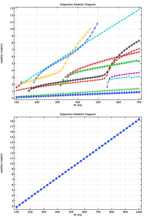
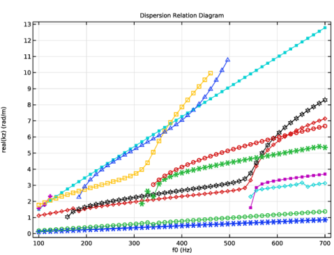
In the Settings window for 1D Plot Group, type Dispersion Relation for Elastic Walls in the Label text field.
3
Click to expand the Title section. From the Title type list, choose Manual.
4
In the Title text area, type Dispersion Relation Diagram.
5
Locate the Data section. From the Dataset list, choose Study 2/Parametric Solutions 1 (sol3).
6
Locate the Plot Settings section.
7
Select the x-axis label checkbox. In the associated text field, type f0 (Hz).
8
Select the y-axis label checkbox. In the associated text field, type real(kz) (rad/m).
9
Locate the Legend section. Clear the Show legends checkbox.
Global 1
1
Right-click Dispersion Relation for Elastic Walls and choose Global.
2
In the Settings window for Global, locate the y-Axis Data section.
3
4
Locate the x-Axis Data section. From the Axis source data list, choose Outer solutions.
5
From the Parameter list, choose Parameter value.
6
Click to expand the Coloring and Style section. Find the Line markers subsection. From the Marker list, choose Cycle.
7
In the Dispersion Relation for Elastic Walls toolbar, click  Plot.
Dispersion Relation for Hard Walls
1
In the Model Builder window, right-click Dispersion Relation for Elastic Walls and choose Duplicate.
2
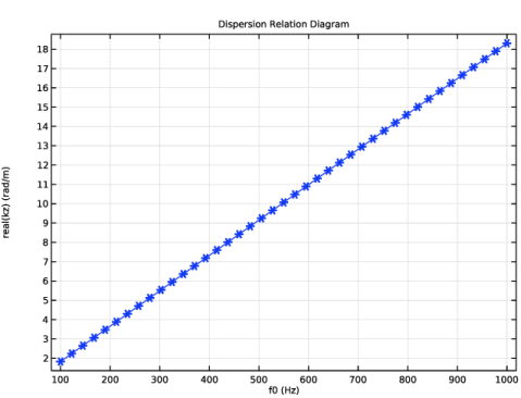
In the Settings window for 1D Plot Group, type Dispersion Relation for Hard Walls in the Label text field.
3
Locate the Data section. From the Dataset list, choose Study 3/Parametric Solutions 2 (sol56).
4
In the Dispersion Relation for Hard Walls toolbar, click  Plot.