PDF

Eigenmodes in Air Bubble with Surface Tension
Introduction
This model analyses the eigenmodes and eigenfrequencies of a spherical air bubble in water. The model evaluates the pulsation mode and a set of surface modes. The eigenfrequencies of the surface modes are determined by the surface tension of the air-water interface. The model compares the numerical results with the analytical results in Ref. 1. Lastly, the impact of the surroundings fluids viscosity on the eigenfrequencies are investigated.
Model Definition
The vibrations of a spherically symmetric bubble are modeled in a 2D axisymmetric model for various azimuthal mode numbers. The model consists of an air bubble with radius = 10 μm in surrounded by a water domain; see Figure 1. The air bubble and surrounding fluid domain is modeled with Thermoviscous Acoustics and then coupled to a Pressure Acoustics domain to which a Spherical Wave Radiation boundary is applied.
The interior boundary condition Surface Tension is used to include the effects of the surface tension on the bubble surface. An eigenfrequency study is used to find the resonances of a 10 μm air bubble in water.
Figure 1: Model geometry of the air bubble (inner circle) and surrounding fluid.
The pulsation or compression resonance of an air bubble in water is given by the sound speed. It therefore depends on whether the pressure field in the bubble is isothermal or adiabatic. For small bubbles the wave will be isothermal and for large bubbles mainly adiabatic. The resonance frequency is given in Ref. 1 as
(1)
where κ is the polytropic coefficient ranging between 1 for isothermal and 1.4 for an isotropic acoustic field, γ is the surface tension coefficient, and P0 is the steady pressure inside the bubble.
The surface modes are governed by the surface tension. If the fluid viscosities are negligible, the resonance frequencies for mode numbers l > 1 are given in Ref. 1 as
(2)
Including the viscosity of the surrounding fluid tends to lower the resonance frequencies. The model investigates mode numbers up to l = 4 and the azimuthal mode numbers m = 0, 1, 2. A resonance mode will be identified by these two mode numbers as (l, m).
When investigating the viscosity the fluid parameters of water will be manipulated such that the viscosity will be
(3)
Where Nμ is a dimensionless scaling parameter and μ0 is the viscosity of water.
Results and Discussion
The resulting pressure field for the eigenmodes will be discontinuous across the air-water interface due to the surface tension. In Figure 2 the pressure field for the mode (= 4, = 0) is shown. Here, l is the total mode number and m is the azimuthal mode number.
Figure 2: Acoustic pressure for the mode (4,0). The pressure is discontinuous across the air-water interface.
The vibrations of the 10 micrometer bubble can be visualized with the Revolving 2D dataset. In Figure 3 the displacement along the normal vector is plotted for the mode (2,2).
.
Figure 3: Color plot of the displacement of the air-water interface for the eigenmode (2,2).
The different eigenmodes correspond to the spherical harmonics. A selection of the modes are shown in Figure 4 for the mode numbers = 0, 2, 3, 4 and azimuthal mode numbers m = 0, 1, 2.
.
Figure 4: The eigenmodes of the air bubble for a set of mode numbers (l, m).
Lastly, the eigenfrequencies are compared to the analytical expressions in Equation 1 and Equation 2. The two red lines show the isothermal and isotropic resonance frequency for the pulsation mode (0, 0) given by Equation 1. The black line show the resonance frequency for the surface modes l = 2, 3, 4 given by Equation 2. Modes with the same wave number but different azimuthal wave number has the same eigenfrequencies. For a negligible viscosity Nμ = 0.02 the eigenfrequencies are in good agreement with the analytical expressions, see Figure 5. For higher viscosity the resonance frequency of the surface modes are decreasing significantly while the resonance of the pulsation mode is constant.
.
Figure 5: Eigenfrequencies for an air bubble in water. The eigenfrequency of the surface modes depends on the viscosity of the surrounding fluid while the pulsation mode is constant.
Notes About the COMSOL Implementation
For the eigenfrequency solver it is important that the equations do not depend on the reciprocal of the frequency. Since the surface tension depends on the displacement of the air-water interface it depends on 1/ω. Therefore, the scaling parameter ta.delta, which is applied to all equations in the Thermoviscous Acoustics interface, is set equal to ta.iomega. Thereby, the equations no longer depend on 1/ω. This is done by setting Equation form to Frequency domain and then setting the scaling factor manually to 1/ta.iomega.
When modeling the azimuthal mode number it is important to set the value in both the Thermoviscous Acoustics and Pressure Acoustics interfaces as well as in the Revolution 2D node under the node Datasets.
Reference
1. S. Temkin, Suspension Acoustics, Cambridge University Press, 2005
Application Library path: Acoustics_Module/Tutorials,_Thermoviscous_Acoustics/eigenmodes_air_bubble
Modeling Instructions
From the File menu, choose New.
New
In the New window, click  Model Wizard.
Model Wizard
1
In the Model Wizard window, click  2D Axisymmetric.
2
In the Select Physics tree, select Acoustics > Thermoviscous Acoustics > Thermoviscous Acoustics, Frequency Domain (ta).
3
Click Add.
4
In the Select Physics tree, select Acoustics > Pressure Acoustics > Pressure Acoustics, Frequency Domain (acpr).
5
Click Add.
6
Click  Study.
7
In the Select Study tree, select General Studies > Eigenfrequency.
8
Global Definitions
Parameters 1
1
In the Model Builder window, under Global Definitions click Parameters 1.
2
In the Settings window for Parameters, locate the Parameters section.
3
Geometry 1
Circle 1 (c1)
1
In the Geometry toolbar, click  Circle.
2
In the Settings window for Circle, locate the Size and Shape section.
3
In the Radius text field, type 8*R0.
4
In the Sector angle text field, type 180.
5
Locate the Rotation Angle section. In the Rotation text field, type -90.
6
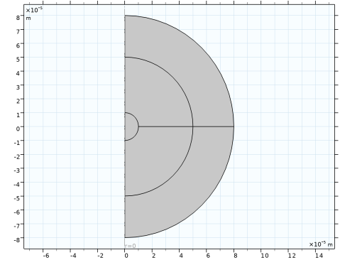
Click to expand the Layers section. In the table, enter the following settings:
7
Click  Build All Objects.
Add Material
1
In the Materials toolbar, click  Add Material to open the Add Material window.
2
Go to the Add Material window.
3
In the tree, select Built-in > Water, liquid.
4
Click the Add to Component button in the window toolbar.
5
In the tree, select Built-in > Air.
6
Click the Add to Component button in the window toolbar.
7
In the Materials toolbar, click  Add Material to close the Add Material window.
Materials
Air (mat2)
Select Domain 3 only.
Water, liquid (mat1)
1
In the Model Builder window, click Water, liquid (mat1).
2
In the Settings window for Material, locate the Material Contents section.
3
The parameter Nmu is introduced to study the resonance frequencies dependency on the viscosity of the surrounding fluid.
Thermoviscous Acoustics, Frequency Domain (ta)
1
In the Model Builder window, under Component 1 (comp1) click Thermoviscous Acoustics, Frequency Domain (ta).
2
In the Settings window for Thermoviscous Acoustics, Frequency Domain, locate the Thermoviscous Acoustics Equation Settings section.
3
Select the Out-of-plane mode extension checkbox.
4
In the m text field, type m.
5
Click to expand the Equation section. From the Equation form list, choose Frequency domain.
6
Locate the Thermoviscous Acoustics Equation Settings section. In the Δ text field, type ta.iomega.
The parameter ta.delta is manually changed so that the final equations do not depend the reciprocal of ta.omega.
Thermoviscous Acoustics Model 1
1
In the Model Builder window, under Component 1 (comp1) > Thermoviscous Acoustics, Frequency Domain (ta) click Thermoviscous Acoustics Model 1.
2
In the Settings window for Thermoviscous Acoustics Model, locate the Model Input section.
3
In the p0 text field, type PAWater.
Thermoviscous Acoustics Model 2
1
In the Physics toolbar, click  Domains and choose Thermoviscous Acoustics Model.
2
3
In the Settings window for Thermoviscous Acoustics Model, locate the Model Input section.
4
In the p0 text field, type PABubble.
5
In the Model Builder window, click Thermoviscous Acoustics, Frequency Domain (ta).
6
Surface Tension 1
1
In the Physics toolbar, click  Boundaries and choose Surface Tension.
2
3
In the Settings window for Surface Tension, locate the Surface Tension section.
4
From the Surface tension coefficient list, choose User defined. In the σ text field, type gamma.
The Surface Tension feature is added on the interior boundary between the air bubble and the surrounding water domain.
Pressure Acoustics, Frequency Domain (acpr)
1
In the Model Builder window, under Component 1 (comp1) click Pressure Acoustics, Frequency Domain (acpr).
2
3
In the Settings window for Pressure Acoustics, Frequency Domain, locate the Pressure Acoustics Equation Settings section.
4
In the m text field, type m.
Pressure Acoustics 1
1
In the Model Builder window, under Component 1 (comp1) > Pressure Acoustics, Frequency Domain (acpr) click Pressure Acoustics 1.
2
In the Settings window for Pressure Acoustics, locate the Model Input section.
3
In the pA text field, type PAWater.
4
Locate the Pressure Acoustics Model section. From the Fluid model list, choose Thermally conducting and viscous.
Spherical Wave Radiation 1
1
In the Physics toolbar, click  Boundaries and choose Spherical Wave Radiation.
2
Multiphysics
Acoustic–Thermoviscous Acoustic Boundary 1 (atb1)
1
In the Physics toolbar, click  Multiphysics Couplings and choose Boundary > Acoustic–Thermoviscous Acoustic Boundary.
2
Mesh 1
Free Triangular 1
In the Mesh toolbar, click  Free Triangular.
Size 1
1
Right-click Free Triangular 1 and choose Size.
2
In the Settings window for Size, locate the Geometric Entity Selection section.
3
From the Geometric entity level list, choose Boundary.
4
5
Locate the Element Size section. Click the Custom button.
6
Locate the Element Size Parameters section.
7
Select the Maximum element size checkbox. In the associated text field, type R0/20.
Size
1
In the Model Builder window, under Component 1 (comp1) > Mesh 1 click Size.
2
In the Settings window for Size, locate the Element Size section.
3
From the Predefined list, choose Fine.
4
Click  Build All.
Study 1
1
In the Model Builder window, click Study 1.
2
In the Settings window for Study, locate the Study Settings section.
3
Clear the Generate default plots checkbox.
Parametric Sweep
1
In the Study toolbar, click  Parametric Sweep.
2
In the Settings window for Parametric Sweep, locate the Study Settings section.
3
From the Sweep type list, choose All combinations.
4
5
6
7
Parametric sweep set up to study different angular mode numbers m and different viscosities.
Step 1: Eigenfrequency
1
In the Model Builder window, click Step 1: Eigenfrequency.
2
In the Settings window for Eigenfrequency, locate the Study Settings section.
3
Select the Desired number of eigenfrequencies checkbox. In the associated text field, type 4.
4
In the Search for eigenfrequencies around shift text field, type 80[kHz].
5
From the Search method around shift list, choose Larger real part.
Solution 1 (sol1)
1
In the Study toolbar, click  Show Default Solver.
2
In the Model Builder window, expand the Solution 1 (sol1) node, then click Eigenvalue Solver 1.
3
In the Settings window for Eigenvalue Solver, locate the General section.
4
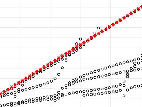
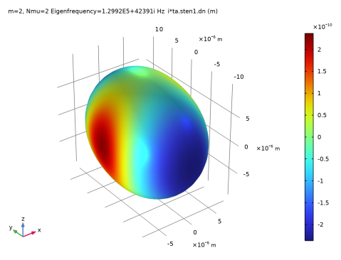
Find the Eigenvalue linearization point subsection. In the Value of eigenvalue linearization point text field, type 250[kHz].
5
In the Study toolbar, click  Compute.
Results
In the Model Builder window, expand the Results node.
Revolution 2D 1
1
In the Model Builder window, expand the Results > Datasets node.
2
Right-click Results > Datasets and choose Revolution 2D.
3
In the Model Builder window, click Revolution 2D 1.
4
In the Settings window for Revolution 2D, locate the Data section.
5
From the Dataset list, choose Study 1/Parametric Solutions 1 (sol2).
6
Click to expand the Revolution Layers section. In the Revolution angle text field, type 380.
7
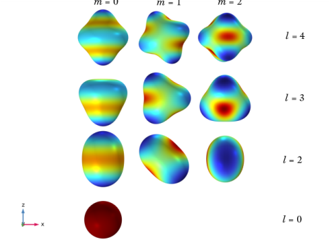
Click to expand the Advanced section. Find the phi subsection. In the Azimuthal mode number text field, type m.
Result Templates
1
In the Results toolbar, click  Result Templates to open the Result Templates window.
2
Go to the Result Templates window.
3
In the tree, select Study 1/Parametric Solutions 1 (sol2) > Acoustic–Thermoviscous Acoustic Boundary 1 > Acoustic Pressure (atb1).
4
Click the Add Result Template button in the window toolbar.
5
In the Results toolbar, click  Result Templates to close the Result Templates window.
Results
Acoustic Pressure (atb1)
1
In the Settings window for 2D Plot Group, locate the Data section.
2
From the Parameter value (m) list, choose 0.
3
From the Parameter value (Nmu) list, choose 1.
4
From the Eigenfrequency (Hz) list, choose 3.8809E5+66550i.
Surface 1
1
In the Model Builder window, expand the Acoustic Pressure (atb1) node, then click Surface 1.
2
In the Settings window for Surface, locate the Expression section.
3
In the Expression text field, type atb1.p_t*i.
4
In the Acoustic Pressure (atb1) toolbar, click  Plot.
Figure of the acoustic pressure for one eigenfrequency with m=0.
Bubble Displacement
1
In the Home toolbar, click  Add Plot Group and choose 3D Plot Group.
2
In the Settings window for 3D Plot Group, type Bubble Displacement in the Label text field.
3
Locate the Plot Settings section. Clear the Plot dataset edges checkbox.
Surface 1
1
Right-click Bubble Displacement and choose Surface.
2
In the Settings window for Surface, locate the Expression section.
3
In the Expression text field, type i*ta.sten1.dn.
4
Locate the Coloring and Style section. From the Scale list, choose Linear symmetric.
Deformation 1
1
Right-click Surface 1 and choose Deformation.
2
In the Settings window for Deformation, locate the Expression section.
3
In the R-component text field, type i*ta.sten1.dn*nr.
4
In the PHI-component text field, type 0.
5
In the Z-component text field, type i*ta.sten1.dn*nz.
6
In the Bubble Displacement toolbar, click  Plot.
Figure of the surface displacement and bubble deformation for one eigenfrequency with m=2.
Bubble Displacement Array
1
In the Home toolbar, click  Add Plot Group and choose 3D Plot Group.
2
In the Settings window for 3D Plot Group, type Bubble Displacement Array in the Label text field.
3
Locate the Plot Settings section. Clear the Plot dataset edges checkbox.
4
Click to expand the Plot Array section. From the Array type list, choose Square.
5
From the Array plane list, choose xz.
Surface 1
1
Right-click Bubble Displacement Array and choose Surface.
2
In the Settings window for Surface, locate the Data section.
3
From the Dataset list, choose Revolution 2D 1.
4
From the Parameter value (m) list, choose 0.
5
From the Parameter value (Nmu) list, choose 1.
6
From the Eigenfrequency (Hz) list, choose 3.0399E5+24043i.
7
Locate the Expression section. In the Expression text field, type i*ta.sten1.dn.
8
Locate the Coloring and Style section. From the Scale list, choose Linear symmetric.
9
Click to expand the Plot Array section. Select the Manual indexing checkbox.
10
In the Row index text field, type 0.
11
In the Column index text field, type 0.
12
Locate the Coloring and Style section. Clear the Color legend checkbox.
13
Click to expand the Title section. From the Title type list, choose None.
Deformation 1
1
Right-click Surface 1 and choose Deformation.
2
In the Settings window for Deformation, locate the Expression section.
3
In the R-component text field, type i*ta.sten1.dn*nr.
4
In the PHI-component text field, type 0.
5
In the Z-component text field, type i*ta.sten1.dn*nz.
Surface 2
1
In the Model Builder window, under Results > Bubble Displacement Array right-click Surface 1 and choose Duplicate.
2
In the Settings window for Surface, locate the Data section.
3
From the Eigenfrequency (Hz) list, choose 1.4169E5+24879i.
4
Locate the Plot Array section. In the Row index text field, type 1.
Surface 3
1
Right-click Surface 2 and choose Duplicate.
2
In the Settings window for Surface, locate the Data section.
3
From the Eigenfrequency (Hz) list, choose 2.5929E5+43471i.
4
Locate the Plot Array section. In the Row index text field, type 2.
Surface 4
1
Right-click Surface 3 and choose Duplicate.
2
In the Settings window for Surface, locate the Data section.
3
From the Eigenfrequency (Hz) list, choose 3.8809E5+66550i.
4
Locate the Plot Array section. In the Row index text field, type 3.
Surface 5
1
Right-click Surface 4 and choose Duplicate.
2
In the Settings window for Surface, locate the Data section.
3
From the Parameter value (m) list, choose 1.
4
From the Eigenfrequency (Hz) list, choose 1.4167E5+24866i.
5
Locate the Plot Array section. In the Row index text field, type 1.
6
In the Column index text field, type 1.
Surface 6
1
Right-click Surface 5 and choose Duplicate.
2
In the Settings window for Surface, locate the Data section.
3
From the Eigenfrequency (Hz) list, choose 2.593E5+43472i.
4
Locate the Plot Array section. In the Row index text field, type 2.
Surface 7
1
Right-click Surface 6 and choose Duplicate.
2
In the Settings window for Surface, locate the Data section.
3
From the Eigenfrequency (Hz) list, choose 3.8806E5+66538i.
4
Locate the Plot Array section. In the Row index text field, type 3.
Surface 8
1
Right-click Surface 7 and choose Duplicate.
2
In the Settings window for Surface, locate the Data section.
3
From the Parameter value (m) list, choose 2.
4
From the Eigenfrequency (Hz) list, choose 1.4169E5+24866i.
5
Locate the Plot Array section. In the Row index text field, type 1.
6
In the Column index text field, type 2.
Surface 9
1
Right-click Surface 8 and choose Duplicate.
2
In the Settings window for Surface, locate the Data section.
3
From the Eigenfrequency (Hz) list, choose 2.5928E5+43459i.
4
Locate the Plot Array section. In the Row index text field, type 2.
Surface 10
1
Right-click Surface 9 and choose Duplicate.
2
In the Settings window for Surface, locate the Data section.
3
From the Eigenfrequency (Hz) list, choose 3.8808E5+66532i.
4
Locate the Plot Array section. In the Row index text field, type 3.
5
In the Bubble Displacement Array toolbar, click  Plot.
6
Click the  Show Grid button in the Graphics toolbar.
7
Click the  Go to XZ View button in the Graphics toolbar.
Array of the pulsation and surface modes for m = 0, 1, and 2.
Evaluation Group 1
In the Results toolbar, click  Evaluation Group.
Global Evaluation 1
1
Right-click Evaluation Group 1 and choose Global Evaluation.
2
In the Settings window for Global Evaluation, locate the Data section.
3
From the Dataset list, choose Study 1/Parametric Solutions 1 (sol2).
4
Locate the Expressions section. In the table, enter the following settings:
5
In the Evaluation Group 1 toolbar, click  Evaluate.
Bubble Resonances
1
In the Home toolbar, click  Add Plot Group and choose 1D Plot Group.
2
In the Settings window for 1D Plot Group, type Bubble Resonances in the Label text field.
3
Locate the Axis section. Select the Manual axis limits checkbox.
4
In the x minimum text field, type 120e3.
5
In the x maximum text field, type 430e3.
6
In the y minimum text field, type -0.05.
7
In the y maximum text field, type 2.05.
Table Graph 1
1
Right-click Bubble Resonances and choose Table Graph.
2
In the Settings window for Table Graph, locate the Data section.
3
From the Source list, choose Evaluation group.
4
From the Plot columns list, choose Manual.
5
From the x-axis data list, choose Eigenfrequency (Hz).
6
In the Columns list box, select Nmu.
7
Locate the Coloring and Style section. Find the Line style subsection. From the Line list, choose None.
8
Find the Line markers subsection. From the Marker list, choose Circle.
Line Segments 1
1
In the Model Builder window, right-click Bubble Resonances and choose Line Segments.
2
In the Settings window for Line Segments, locate the x-Coordinates section.
3
4
Locate the y-Coordinates section. In the table, enter the following settings:
5
Click to expand the Coloring and Style section. From the Color list, choose Black.
6
In the Bubble Resonances toolbar, click  Plot.
Line Segments 2
1
Right-click Bubble Resonances and choose Line Segments.
2
In the Settings window for Line Segments, locate the x-Coordinates section.
3
4
Locate the y-Coordinates section. In the table, enter the following settings:
5
Click to expand the Coloring and Style section. From the Color list, choose Black.
6
In the Bubble Resonances toolbar, click  Plot.
Line Segments 3
1
Right-click Bubble Resonances and choose Line Segments.
2
In the Settings window for Line Segments, locate the x-Coordinates section.
3
4
Locate the y-Coordinates section. In the table, enter the following settings:
5
Click to expand the Coloring and Style section. From the Color list, choose Black.
Plotting the theoretical eigenfrequencies for an inviscid surrounding fluid.
Line Segments 4
1
Right-click Bubble Resonances and choose Line Segments.
2
In the Settings window for Line Segments, locate the x-Coordinates section.
3
4
Locate the y-Coordinates section. In the table, enter the following settings:
5
Click to expand the Coloring and Style section. From the Color list, choose Red.
Line Segments 5
1
Right-click Bubble Resonances and choose Line Segments.
2
In the Settings window for Line Segments, locate the x-Coordinates section.
3
4
Locate the y-Coordinates section. In the table, enter the following settings:
5
Click to expand the Coloring and Style section. From the Color list, choose Red.
Plotting the theoretical eigenfrequencies for the surface modes (black) and the analytical prediction for the pulsating mode for an adiabatic and isothermal acoustic field (red).
6
In the Bubble Resonances toolbar, click  Plot.